 Copper
The evaluation of copper concentrations in various compartments of the Baltic Sea marine environment has both ecological and policy relevance.
2.1 Ecological relevance
Copper is an essential element for organisms but is toxic to marine species when concentrations exceed levels that are physiologically required (Campbell, 1995). Copper is accumulated by plants and animals. At high concentrations, copper becomes toxic, as it affects the metabolic processes of marine organisms. In addition to acute effects (e.g. mortality), chronic exposure to copper can lead to adverse effects on survival, growth and reproduction of individual organisms. This may in turn transform into changes at species and population level, impacting biodiversity and ecosystem health.
2.2 Policy relevance
The core indicator directly addresses the Baltic Sea Action Plan (BSAP) Hazardous substances and litter segment goal of a ‘Baltic Sea unaffected by hazardous substances and litter’. In addition, it also has relevance for aspects of the biodiversity segment.
The indicator is also applicable for the EU Marine Strategy Framework Directive (MSFD), in particular addressing Descriptor 8 – Concentrations of contaminants are at levels not giving rise to pollution effects. Other MSFD descriptors and criteria are also relevant such as those addressing biodiversity and pelagic habitats (Descriptor 1), those addressing ecosystems/food webs (Descriptor 4) and also those addressing benthic habitats (Descriptor 6).
An overview of policy relevance is provided in the Table 1.
Table 1. Policy relevance of the copper indicator.
| Baltic Sea Action Plan (BSAP) | Marine Strategy Framework Directive (MSFD) | |
| Fundamental link | Segment: Hazardous substances and litter goal
Goal: “Baltic Sea unaffected by hazardous substances and litter”
|
Descriptor 8 Concentrations of contaminants are at levels not giving rise to pollution effects.
|
| Complementary link |
|
Descriptor 8 Concentrations of contaminants are at levels not giving rise to pollution effects.
Element of the feature assessed – Species list. Descriptor 9 Contaminants in fish and other seafood for human consumption do not exceed levels established by Union legislation or other relevant standards.
(a) for contaminants listed in Regulation (EC) No 1881/2006, the maximum levels laid down in that Regulation, which are the threshold values for the purposes of this Decision; (b) for additional contaminants, not listed in Regulation (EC) No 1881/2006, threshold values, which Member States shall establish through
Descriptor 1 Species groups of birds, mammals, reptiles, fish and cephalopods.
Descriptor 6 Sea-floor integrity is at a level that ensures that the structure and functions of the ecosystems are safeguarded and benthic ecosystems, in particular, are not adversely affected.
|
| Other relevant legislation: |
|
|
2.3 Relevance for other assessments
Each hazardous substances HELCOM indicator addresses a specific substance of group of substances with potential negative impacts on the Baltic Sea ecosystem. This copper indicator also adds to the evaluation of metals concentrations in the Baltic Sea, in addition to the evaluation of cadmium, lead and mercury. The Copper indicator will be included in the integrated hazardous substances assessment, using the HELCOM hazardous substances assessment tool CHASE.
Good Status is achieved if the concentrations of copper are below the specified threshold value, see schematic representation (Figure 2).
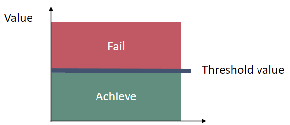
Figure 2. Schematic representation of the threshold value applied in the Copper core indicator (the threshold value is presented in the table below).
The threshold value applied is an Environmental Quality Standard (EQS) for sediment and utilised on a dry weight basis inclusive of a total organic carbon (TOC) correction factor to account for bioavailability (see Table 2). The threshold value was approved for regional application by HOD 61-2021 (see document 5-1 Rev.1 and associated workspace).
Table 2. Threshold value for copper (EQS – Environmental Quality Standard).
| Substance evaluated | Matrix | Threshold value | Reference |
| Copper (in all assessment units) | Sediment | 30 mg/kg d.w. (5% TOC) | EQSsediment |
3.1 Setting the threshold value
The methodology and approach to derive a threshold value for copper in Baltic Sea sediment is described in detail in the technical report by Lagerström et al. (2021), commissioned by the Swedish Agency for Marine and Water Management. The EQS-values of copper in use by different HELCOM Contracting Parties differ by a factor of up to 50 (Lagerström et al., 2021). The main reasons for the substantial differences in national EQS for sediment and water originates from different assumptions regarding bioavailability, natural background, as well as quality assessment and data treatment of available ecotoxicological data. To discuss and hopefully resolve some of these issues, Chalmers University of Technology, together with the Swedish Agency for Marine and Water Management and the Danish Ministry of Environment organised three workshops in the spring of 2021. The workshop series was entitled “Towards a harmonised approach for the derivation of an EQS for copper in marine sediments”. Participants were experts representing academia, industry, consulting agencies and governmental authorities. Three main topics were discussed: 1) bioavailability, 2) natural background and 3) how ecotoxicological data should be treated when deriving an EQS for copper in marine sediments. The main objective of this expert elicitation endeavour was to provide concrete suggestions on each of the three topics, combining both scientific knowledge and practical feasibility. Details on each of the workshops, as well as all group discussion notes can be found in Lagerström et al. (2021), Appendix A.
Approach to derive the threshold value
The process of deriving a threshold value for copper in sediment was separated into two parts. The first part was focused on collecting input from several sectors and expert judgement on methodology through three workshops. The second part consisted of an extensive literature study where ecotoxicological data was collected for further analysis. The Technical Guidance Document No. 27 (European Commission, 2018), hereafter TGD 27, served as a starting point for deriving the EQS of copper in sediment and has been used as the main supporting guidance document during decision making. When guidance on derivation of metals in the sediment matrix were lacking, expert judgement and interpretation from guidance of deriving EQS in the water matrix have also been important.
To account for bioavailability, normalisation to organic carbon can be justified if it reduces the variability in the dataset. This is stated in TGD 27 and was also supported by participants at Workshop 1 on bioavailability and Workshop 3 on ecotoxicological data and EQS derivation. TGD 27 suggests that background concentrations should be assessed during the implementation of the EQS rather than during the derivation process. This was also supported by participants at workshop 2. A decision to use the total risk approach (TRA), rather than the added risk approach (ARA) was therefore applied for the EQS derivation. At workshop 3, participants expressed a clear preference for a probabilistic approach over a deterministic one. A probabilistic approach (i.e. an SSD – species sensitivity distribution) was therefore selected to derive the HC5 (i.e. the concentration where 5% of the species included are affected). Since the Baltic Sea has a unique environment consisting of freshwater, brackish and marine species, participants at workshop 3 suggested that pooling of freshwater and marine ecotoxicological data could be appropriate. Additionally, this would provide a more extensive dataset allowing the application of the preferred probabilistic approach.
SSD analysis and estimation of HC5
Ecotoxicological studies and data was compiled from previous EQS dossiers (e.g. European Copper Institute, 2008; Sahlin and Ågestrand, 2018) and complemented with newer studies on the toxicity of copper in marine and freshwater sediments. The ecotoxicological data and studies used to derive an EQS for copper (including the reliability and relevance assessment) are described in detail in Lagerström et al. (2021), Appendix B. In accordance with TGD 27, a statistical two tailed t-test (assuming unequal variances (F-test confirmation)) between the marine and freshwater datasets confirmed that pooling of the data was supported. There was no significant difference between freshwater and marine NOEC/EC10 values (p=0.36 non-normalised data and p=0.64 for TOC-normalised data). The final dataset of ecotoxicological test results represented a total of 12 species from 9 taxonomic groups (on order level) (Figure 3). The dataset included 4 marine species (4 taxonomic groups) and 8 freshwater species (5 additional taxonomic groups + amphipoda already represented by marine species) where the species represent different feeding and living conditions from both the marine and limnic environment (Figure 3, and more detailed description in Lagerström et al. (2021), Appendix B).
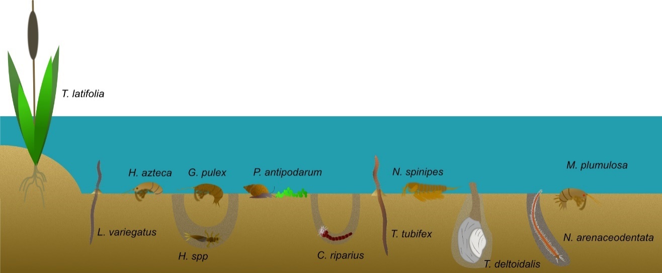 Figure 3. Feeding/living conditions of species included in the final SSD analysis. The four species to the right (N. spinipes, T.deltoidalis, N. arenaceodentata and M. plumulosa) were tested in marine sediments whereas the others were tested in freshwater sediments.
Prior to the SSD analysis, the data was normalised to 5% (total) organic carbon. Based on the calculations of Max:Min ratios of the different species-specific endpoints it could be argued that the variability within the dataset was reduced by normalisation to organic carbon. A comparison of the relative standard deviations (RSDs) for 6 species and endpoints also showed a decrease when data was normalised to organic carbon (Lagerström et al. (2021) and Table 1 in Appendix B). Based on this, it was decided to normalise the data to 5% organic carbon (following TGD 27 recommendations) prior to the SSD analysis.
As TGD 27 highlights the importance of using worst-case scenario ecotoxicological tests, and that the acid volatile sulphides (AVS) can reduce the bioavailability and thus increase the apparent tolerance of copper in sediment, studies with high AVS levels were removed from the final SSD analysis. Most studies where AVS > 1 μmol/g were thus excluded from the dataset to follow TGD 27 recommendations. However, several of the ecotoxicology studies on marine species were conducted under conditions where AVS is defined as being <4.5 μmol/g (see Appendix B), but as these tests included some of the more sensitive species and endpoints they were nonetheless included in the final analysis. Where no information on AVS was provided, expert judgement considering oxygen supply, redox potential and sediment origin determined whether or not the test results were included in the final SSD.
SSD analysis was conducted using the US-EPA SSD toolbox (US-EPA, 2020), allowing for several different fitting methods and distribution functions that could be compared to obtain the best fit for the available data (see Lagerström et al. (2021), Appendix B). Maximum likelihood was used as the fitting method for all analysis as this is a commonly applied and preferred approach when performing SSD for regulatory purposes (Carr and Belanger, 2019; Fox et al., 2021). The final dataset consisted of 49 test results (NOEC and EC10 values) from 12 species. The logistic distribution offered the best fit (Appendix B for comparison), with an overall R2 value of 0.97 (Q-Q plot, Figure 4). Despite this, the generated HC5 value (61 mg/kg dw) is not protective of the most sensitive species/endpoints of M. plumulosa (40 mg/kg dw), H. Azteca (51 mg/kg dw), T. tubifex (32 mg/kg dw) and T. deltoidalis (37 mg/kg dw). Applying the logistic distribution, the derived HC5=61 mg/kg dw (Lower limit 33 mg/kg; upper limit 124 mg/kg) (Figure 4).
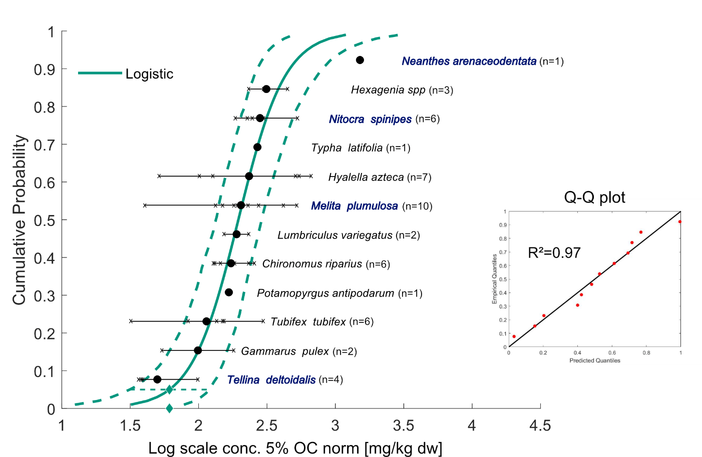
Figure 4. The log logistic SSD curve based on NOEC/EC10 values normalised to 5% organic carbon. The dots represent the geometric mean (or single value) of each species (written to the right of the curve, dark blue and bold show marine species) with the horizontal line representing the range and the cross symbols (x) showing the discrete NOEC/EC10 value for each species (number of values=n). The full line represents the fitted curve while the dashed lines show the upper and lower confidence interval of the fitting of the curve. The diamond shows the HC5 value (and is also put on the x-axis for better read) and the horizontal dashed line shows the 95% confidence interval of the HC5 value. The inset “Q-Q plot” represents the goodness-of-fit of the curve where the R2 value=0.97.
Derived threshold value
The derived HC5 value was used to calculate a protective EQS value for copper in sediments for the Baltic Sea region by dividing the HC5 value with an additional safety factor, also known as assessment factor (AF). To set an appropriate AF, several aspects were considered in the weight-of-evidence approach suggested by TGD 27. In the report by Lagerström et al. (2021) an AF of 3 was proposed. However, due to uncertainties in natural background concentrations of copper in sediment, the contracting parties of HELCOM agreed to use an AF of 2, yielding an EQSsediment = 30 mg/kg d.w. normalised to 5% TOC (HELCOM HOD 61-2021, document 5-1 Rev.1).
The results of the indicator evaluation that underlie the key message map and information are provided below.
4.1 Status evaluation
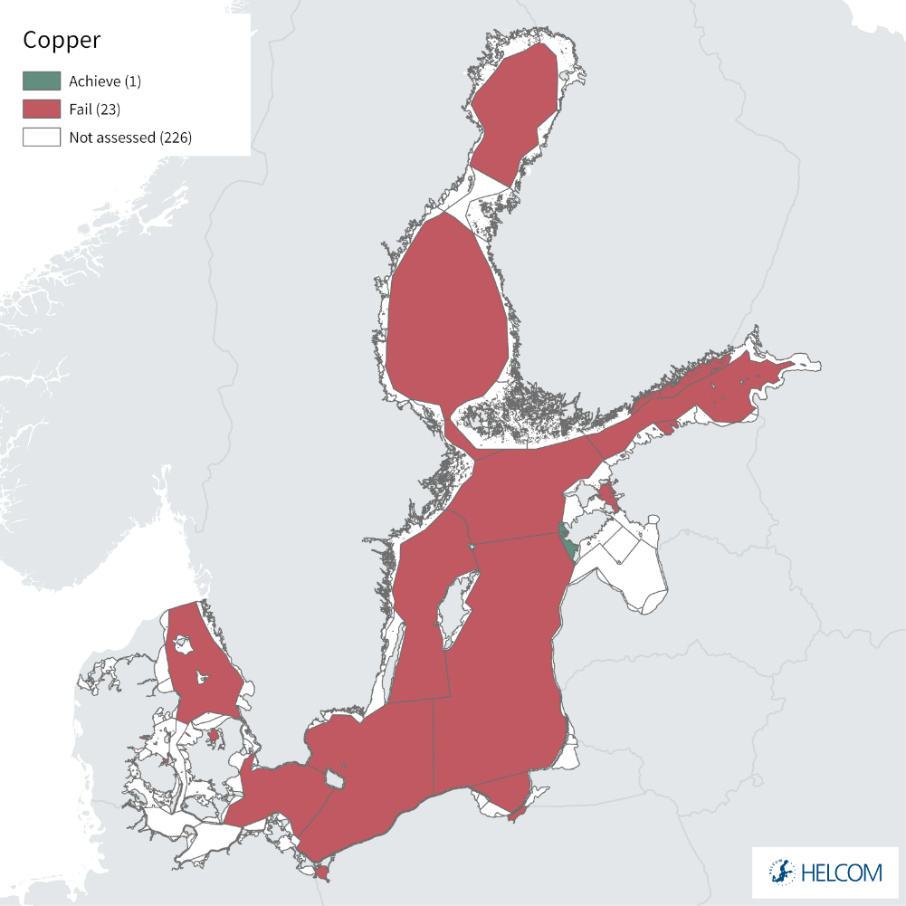
The threshold value is not achieved, thus indicating a sub-Good Environmental Status (sub-GES) condition, in all but one of the assessment units evaluated (Figure 5 and Figure 6). All 11 evaluated open sea sub basins fail to achieve the threshold value and of the 13 coastal assessment units evaluated only one, EST-011 (Estonia – Kihelkonna Bay CWB) located in the northerly edge of the Eastern Gotland Basin achieved GES. In a number of assessment units the threshold is exceeded by a large margin.
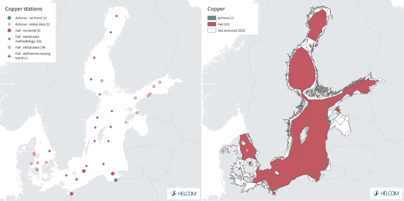
Figure 5. Map presenting station based status of copper concentrations in sediment (left) and assessment unit based status for copper in sediment (right). Green colour represents good status and red colour represents not good status. See ‘data chapter’ for interactive maps and data at the HELCOM Map and Data Service.
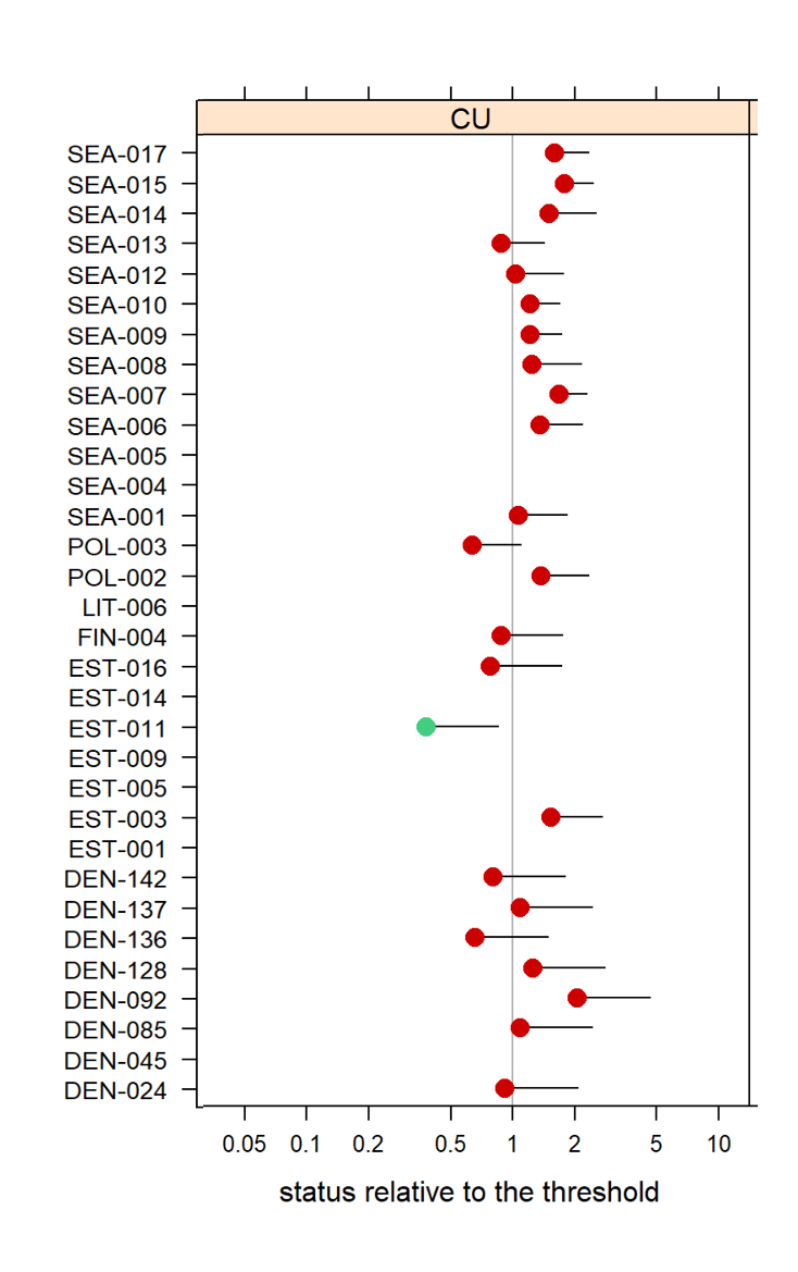
Figure 6. Status evaluation, relative to threshold value, in the assessment units evaluated. Circles represent a mean value for each assessment unit and the bar represents the upper 95% confidence limit. Green colour indicates that the assessed area achieves the threshold value and red colour that the assessed area fails the threshold. Note that not all assessment units in the figure above are evaluated (see also table below).
4.2 Trends
Of the 35 stations that provided sufficient data (and supporting parameters) to carry out an evaluation, and are thus incorporated into the assessment unit level status evaluation presented above, 20 stations contained ‘full’ data series (more than 2 years of data) and 15 ‘initial’ data series (1-2 years of data). Two of these stations achieved GES and the remainder were sub-GES, though when integrated at the assessment unit level one of the stations was outweighed by other sub-GES stations. Where statistical trends are applied (i.e. for full data series) stable or no trends were detected in all but one case. This is in part due to variation in the data series between sampling years. In one case, the Polish Bornholm Basin station PL-P39, a distinct increasing trend was recorded (i.e. suggesting concentrations appear to be increasing, see Figure 5). However, this trend is uncertain as the measured concentrations from 2007 to 2018 appears to be rather constant and in the range of 30 to 40 mg/kg (dry weight sediment) normalised to 5% TOC. A series of example time trends from the analyses are provided in Figure 7.
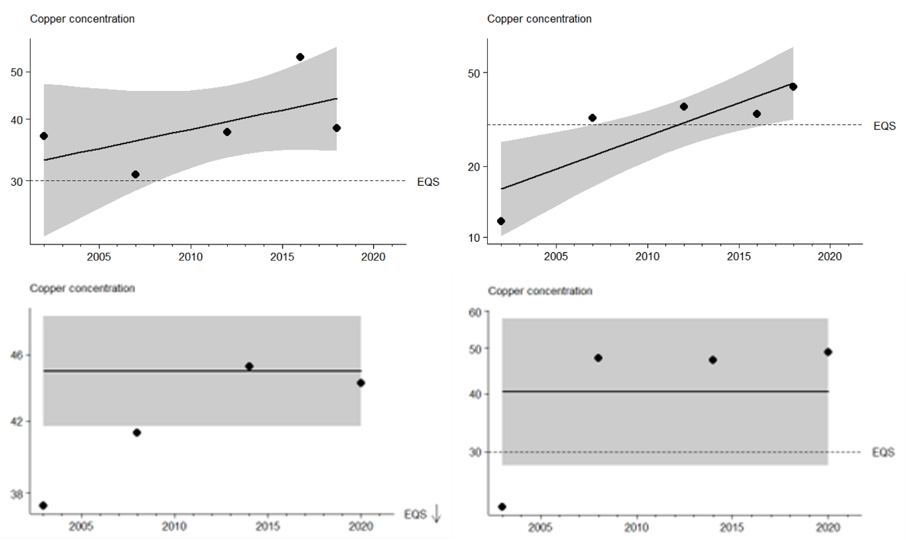
Figure 7. Example trends for selected stations where more detailed time series data (‘full’ data ) are available. Top left: PL-P5C (Poland, Bornholm Deep – ‘full data’ no distinct trend); Top right: PL-P39* (Poland, Bornholm Basin – ‘full data’ distinct upward trend (increasing concentration)); Bottom left: SE-4 (Sweden, Åland Deep); and Bottom right: SE-17 (Sweden, N Bothnian Bay).*this station records an increasing trend in the analyses.
4.3 Discussion text
The indicator is evaluated in the majority of open sea assessment units, where the outcomes is evaluated as sub-GES. Relatively few coastal assessment units are evaluated though in areas where an evaluation was possible, sub-GES status was generally recorded. This indicator is new in HOLAS 3 and is therefore the first iteration of the status evaluation, consequently no comparisons can be made with prior evaluations. An overview of the status information is provided in table 3.
Table 3. Overview of status evaluation outcomes.
| HELCOM Assessment unit name (and ID) | Threshold value achieved/failed – HOLAS 2 | Threshold value achieved/failed – HOLAS 3 | Distinct trend between current and previous evaluation. | Description of outcomes, if pertinent. |
| Kattegat (SEA-001) | NA | Failed | NA – no previous evaluation made | The threshold value is not achieved thus the evaluation is sub-GES. The evaluation is based on a low number of detailed time series (‘full data’). |
| Arkona Basin (SEA-006) | NA | Failed | NA – no previous evaluation made | |
| Bornholm Basin (SEA-007) | NA | Failed | NA – no previous evaluation made | |
| Gdansk Basin (SEA-008) | NA | Failed | NA – no previous evaluation made | |
| Eastern Gotland Basin (SEA-009) | NA | Failed | NA – no previous evaluation made | |
| Western Gotland Basin (SEA-010) | NA | Failed | NA – no previous evaluation made | |
| Gulf of Riga (SEA-012) | NA | Failed | NA – no previous evaluation made | |
| Gulf of Finland (SEA-013) | NA | Failed | NA – no previous evaluation made | The threshold value is not achieved thus the evaluation is sub-GES. The evaluation is based on a moderate number of ‘initial’ time series. |
| Åland Sea (SEA-014) | NA | Failed | NA – no previous evaluation made | The threshold value is not achieved thus the evaluation is sub-GES. The evaluation is based on a low number of detailed time series (‘full data’). |
| 015 Bothnian Sea (SEA-015) | NA | Failed | NA – no previous evaluation made | The threshold value is not achieved thus the evaluation is sub-GES. The evaluation is based on a moderate number of detailed time series (‘full data’) and an initial data series. |
| Bothnian Bay (SEA-017) | NA | Failed | NA – no previous evaluation made | The threshold value is not achieved thus the evaluation is sub-GES. The evaluation is based on a moderate number of detailed time series (‘full data’). |
| Isefjord, ydre (DEN-024) | NA | Failed | NA – no previous evaluation made | The threshold value is not achieved thus the evaluation is sub-GES. The evaluation is based on a low number of ‘initial’ time series. |
| Kertinge Nor (DEN-085) | NA | Failed | NA – no previous evaluation made | |
| Odense Fjord, ydre (DEN-092) | NA | Failed | NA – no previous evaluation made | |
| Horsens Fjord, indre (DEN-128) | NA | Failed | NA – no previous evaluation made | |
| Randers Fjord, indre (DEN-136) | NA | Failed | NA – no previous evaluation made | |
| Randers Fjord, ydre (DEN-137) | NA | Failed | NA – no previous evaluation made | |
| Stavns Fjord (DEN-142) | NA | Failed | NA – no previous evaluation made | |
| Hara Bay CWB (EST-003) | NA | Failed | NA – no previous evaluation made | |
| Kihelkonna Bay CWB (EST-011) | NA | Achieved | NA – no previous evaluation made | The threshold value is achieved thus the evaluation is in GES. The evaluation is based on a low number of ‘initial’ time series. |
| Väinamere CWB (EST-016) | NA | Failed | NA – no previous evaluation made | The threshold value is not achieved thus the evaluation is sub-GES. The evaluation is based on a low number of ‘initial’ time series. |
| Suomenlahden ulkosaaristo (FIN-004) | NA | Failed | NA – no previous evaluation made | |
| PL TW I WB 8 (POL-002) | NA | Failed | NA – no previous evaluation made | |
| PL TW I WB 1 (POL-003) | NA | Failed | NA – no previous evaluation made |
The overall confidence of the evaluation is considered to be moderate to high (see Figure 8, and table in Annex 1). The evaluated assessment units were categorized as having moderate overall confidence with the exception of SEA-010 (Western Gotland Basin) which was evaluated overall as having high confidence (methodological details are provided in Annex 1).
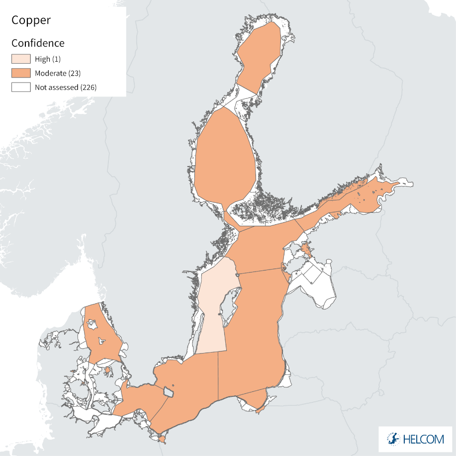
Figure 8. Map presenting the overall confidence in the status evaluation of copper concentrations in sediment.
The methodology applied to derive the threshold value is based on TGD 27 and from expert elicitation workshops. The threshold value is derived based on a probabilistic approach using an SSD curve, where the dataset comprises of 4 marine species and 8 freshwater species representing different feeding and living conditions. However, no ecotoxicological data on Baltic species were available. The probabilistic approach is preferred over the deterministic approach since the deterministic approach holds higher uncertainties with an assessment factor typically in the range of 10-1000 is applied. The confidence of the threshold value is hence considered to be high. In addition the methodology applied to carry out the evaluation utilizes the regionally agreed MIME assessment script, the basis of which is identical to tools used on the North Atlantic (OSPAR). Thus, overall methodological confidence is scored as high.
The confidence in the status evaluation is however considered to be moderate, due to uncertainties in how to account for local background concentrations of copper. If sediment concentrations are near the threshold value (or in exceedance), it is recommended that local natural concentrations should be defined to evaluate if the target of near natural background of copper is met locally and whether further measures are appropriate. This matter is described more in detail below, see chapter 5.1. To improve the areas of uncertainty, future work could include ecotoxicological studies on Baltic Sea species, broader overview of sediment background concentrations in the different Baltic Sea basins, including content of organic carbon.
5.1 Consideration of natural background concentrations
TGD 27 specifies that the size of the AF should not normally result in a quality standard below typical natural background concentration (NBC). This is particularly stressed for metals. Studies on the background concentrations of copper in the Baltic Sea are however currently lacking. Nonetheless, to attempt to evaluate whether an AF of 2 would lead to an EQS < NBC, the sediment data set presented in Lagerström et al. (2021), section 1.2.2, was searched for samples collected at depths below 10 cm. A total of 17 stations, of which some had been sampled recurringly, were found. As shown by the map in Figure 9, the stations were located in 8 different subbasins of the southern Baltic Sea. Hence, no deep samples for the northern and eastern Baltic Sea (e.g. Gulf of Finland) were part of this analysis. Although the sediments have not been dated, the plotted profiles show that the concentrations typically vary little at depths below 15-20 cm. The concentration in such deep samples could thus give an idea of the range of background concentrations of Cu in the Baltic Sea. Below 20 cm, concentrations of Cu (not normalized to TOC) are typically between 10-50 mg/kg, dw, except for the Eastern Gotland Basin where concentrations as high as nearly 100 mg/kg dw have been measured.
However, when assessing the applicability of the proposed EQS (which is normalized to 5 % TOC), it could also be argued that the background concentrations should be normalised to 5% TOC. TOC concentrations were only reported for sediment samples from 3 of the 8 subbasins (Figure 10). At depths of 30 cm, the normalised concentrations in the three subbasins (Bornholm Basin, Eastern Gotland Basin and Gdansk Basin) range from 4.3 to 23.3 mg/kg dw, with an average ± 1 standard deviation of 13.6 ± 4.6 mg/kg dw (5% TOC normalisation). These results suggest that the NBC in these subbasins is below the proposed EQS value of 30 mg/kg dw, at 5% TOC. More studies in different HELCOM subbasins and preferably with dating of the sediments are however needed to allow for a more accurate determination of the NBC. If such studies would reveal that an EQS based on an AF of 2 is indeed below the NBC, TGD 27 states the first step is to investigate how to reduce the uncertainty of the EQS. If the uncertainty cannot be reduced, for example through additional ecotoxicological studies, the natural background can be taken into account when assessing compliance. In locations where the EQS value exceeds the natural background, the natural background could for instance be used as the threshold value instead, as proposed by the experts participating in the workshop organized by Lagerström et al. (2021), see Appendix A.
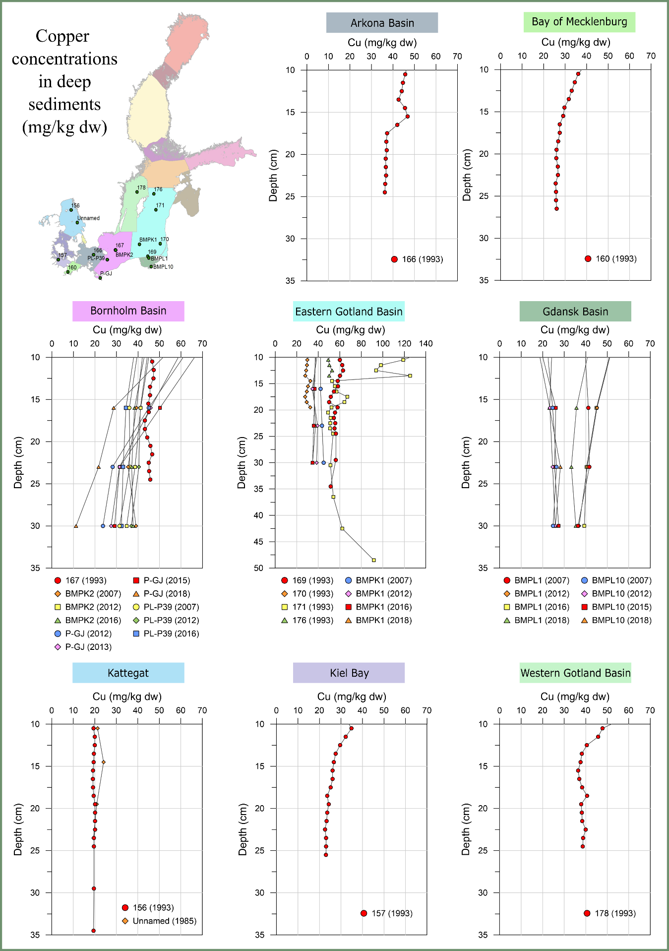 Figure 9. Sediment depth profiles with sampling depths > 10 cm. The scales of the x- and y-axis’s are the same for all graphs except the Easter Gotland Basin. Note that some of the stations were sampled several years and that the information presented here is not normalised to 5% TOC.
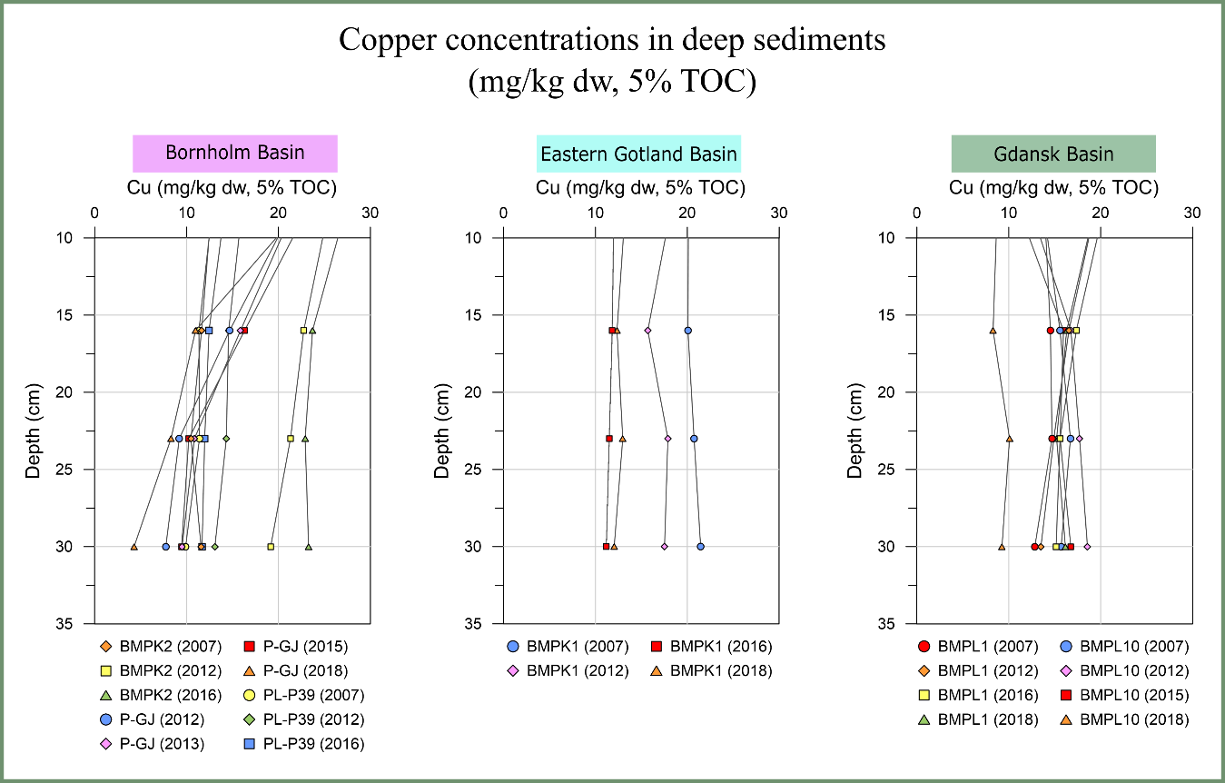 Figure 10. Sediment depth profiles with sampling depths > 10 cm, normalised to 5% organic carbon. See Lagerström et al. (2021) for more details.
Drivers are often large and disparate entities that are hard to identify and quantify, for example globalization, consumer trends or political will. To identify drivers and attempt to evaluate and qualify/quantify them, the use of proxies is often useful. Drivers motivate changes in activities and thereby alter pressures such as inputs of substances to the marine environment. A brief overview is provided in Table 4.
Table 4. Brief summary of relevant pressures and activities with relevance to the indicator.
| | General | MSFD Annex III, Table 2a |
| Strong link | Shipping, marine infrastructure, and certain industrial operations can all contribute to releases of copper to the marine environment. | Substances, litter and energy
|
| Weak link |
Inputs of Cu to the Baltic Sea can be of natural origin (e.g. leaching from forest and other land areas) or from anthropogenic sources (e.g. antifouling paint and industries). Load estimations of Cu to the Baltic Sea from natural sources and human activities have been compiled by Ytreberg et al. (2022). The compilation included the following activities/sources: atmospheric deposition, riverine inputs, point sources (i.e. coastal industries and wastewater treatment plants), shipping and leisure boating (Figure 11).
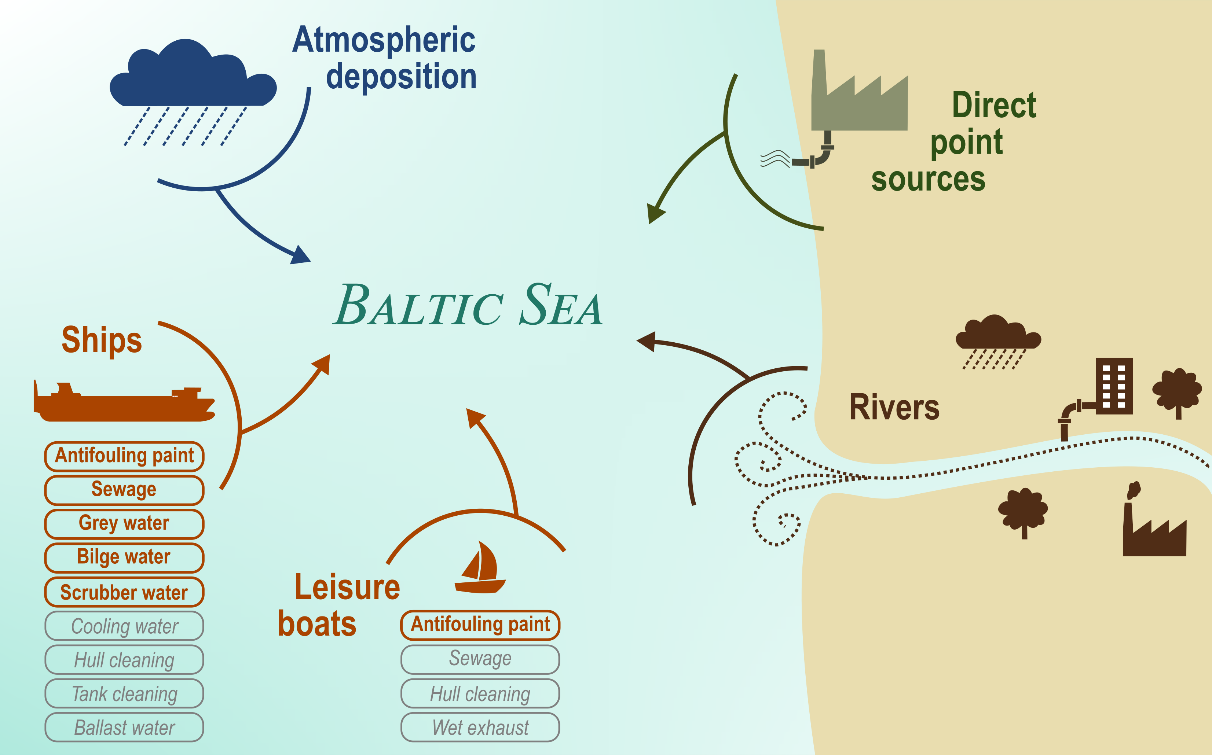
Figure 11. Activities and pressures of copper considered in Ytreberg et al. (2022). Grey text in italic indicates sources where data is lacking and thus not included in the assessment.
The results of earlier analyses show that the total annual load of Cu to the Baltic Sea, derived for 2018, to be 1560 tonnes (t), of which riverine input contributed to 54 % of the total input (850 t) (Figure 12). Emissions from Danish rivers is excluded in the compilation due to data gaps. To what extent the riverine input of Cu to the Baltic Sea originates from natural or anthropogenic sources is unknown. However, some guidance can be obtained from a Swedish study by Ejhed et al. (2010), where point sources and diffuse emissions of Cu to Swedish catchment areas (inland waters) from various sources were compiled based on data from 1985 to 2004. The results showed the total diffusive emissions of Cu to Swedish inland waters to be 156 t/year. The emissions are divided into leaching from forest land (52 t/year, 34%), stormwater from urban areas and roads (38 t/year, 25%), leaching from agriculture (30 t/ year, 19%), leaching from remaining land areas (21 t/year, 14%) and atmospheric deposition on lakes (14 t/year, 9%). The total emissions to Swedish catchment areas from point sources are much lower with a total of 35 t/year where industries and wastewater treatment plants respectively accounted for 21 and 11 t/year (Ejhed et al., 2010). The extent to which this total Cu load from point and diffusive sources to Swedish inland waters (in total 190 t/year) contributes to the load to the Baltic Sea via rivers is however unknown.
The second largest source of Cu to the Baltic Sea is maritime shipping and leisure boating, which together account for 37 % of the load (575 t) (Figure 12). The largest share (98 %) of the Cu load from shipping and leisure boating is from antifouling paints, where shipping and leisure boating annually account for 509 and 57 t, respectively. Globally, Cu (as cuprous oxide) is the dominating biocide in antifouling paints (Amara et al., 2018), but the release rate from the coating to the ambient water can vary between products from 2 to 66 µg/cm2/day (Jalkanen et al., 2021). Notably, the form (chemical species) in which Cu is released from antifouling paint is different as compared to most other sources. For example, calculation of Cu speciation in rivers indicates that forms of Cu complexed by organic matter predominate substantially over bioavailable free or inorganic forms of the metal (Gardner et al., 2000). For antifouling paints, the situation is the reverse: Sandberg et al. (2007) found that 80% of the leached Cu from antifouling coatings was in bioavailable form during a laboratory study with artificial seawater. A field study has also shown the proportion of dissolved Cu in bioavailable form in a Baltic Sea marina to more than double during the boating season as a result of the use of antifouling coatings (Lagerström et al., 2020). As the evaluation of the copper indicator involves normalisation to organic carbon, the inputs of copper from antifouling paints thus have a greater potential to negatively impact the indicator compared to riverine input.
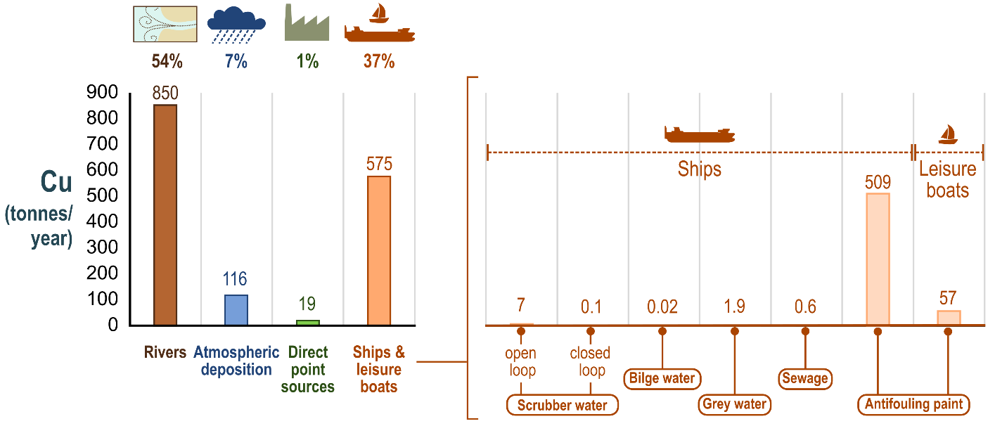
Figure 12. Estimated load of copper to the Baltic Sea in 2018, from Ytreberg et al. (2022).
As shown in Table 5, the load of copper from shipping is primarily concentrated to the basins Baltic Proper (213 t), Gulf of Finland (110 t), Danish Straits (80 t) and Kattegat (66 t). The share of Cu from shipping is highest in Danish Straits (81%), Kattegat (62%) and Baltic Proper (55%). It should however be emphasized that the input from leisure boats and point sources is not included in this basin assessment due to the lack of spatial distributed input of Cu from these activities, and as mentioned previously, emissions of Cu from Danish rivers are lacking.
Table 5. Load of copper in Baltic Sea basins, from Ytreberg et al. (2022). Highlighting is applied to sources and sub-basins where loads are relatively high (orange shades) or relatively low (blue shades).
| Input source | Bothnian Bay | Bothnian Sea | Baltic Proper | Gulf of Finland | Gulf of Riga | Danish Straits | Kattegat | All basins |
| Ships | 12 | 27 | 213 | 110 | 10 | 80 | 66 | 518 |
| Leisure boats | 57 | |||||||
| Riverine input | 150 | 100 | 120 | 390 | 60 | 5.4 | 30 | 850 |
| Point sources | 19 | |||||||
| Atmospheric deposition | 8.0 | 12 | 57 | 8.2 | 5.0 | 14 | 11 | 116 |
| All sources | 170 | 139 | 390 | 508 | 75 | 99 | 107 | 1560 |
7 Climate change and other factors
Copper does not degrade in the environment, but changes in environmental parameters from climate change can act to increase or decrease its bioavailability and thus affect the potential for the copper indicator to achieve good status in the future. Additionally, climate change may impact the sources of copper to the Baltic Sea. The impact of climate change on the copper indicator must therefore consider both its effect on copper bioavailability but also on the emission sources themselves.
As a result of increased precipitation, river run-off to the Baltic Sea has been projected to increase from present day by 2-22% with warming temperatures (HELCOM, 2021). This increase will take place mostly in the North as the increase in precipitation is expected to be largest here. The South may instead experience potentially decreasing total runoff. Riverine inputs of copper to the Baltic Sea may therefore increase, particularly in the Bothnian Bay and Bothnian Sea. The predicted increased sedimentation from coastal erosion may also act to increase inputs of copper in coastal areas (HELCOM, 2021). However, as increased freshwater discharge would also bring more dissolved organic carbon to the sea which acts to reduce the bioavailability of copper, it is not clear whether the effect of increased run-off would affect the status of the copper indicator negatively. Increased sedimentation due to both increased river run-off and coastal erosion may also increase the dredging demand of marinas and ports where sediments tend to be contaminated with high concentrations of copper (Staniszewska and Boniecka, 2017; 2018). However, the potential increased need of dredging may be mitigated by sea level rise (HELCOM, 2021).
Baltic Sea water temperatures are projected to increase with the warming climate (HELCOM, 2021). This will likely affect the copper emissions from antifouling coatings which have been identified as the second largest sources of copper to the Baltic Sea next to riverine input (Figure 10). Copper compounds currently added to antifouling coatings include cuprous oxide, copper thiocyanate, copper powder and copper pyrithione (Paz-Villarraga et al., 2021). Of these, cuprous oxide is the most commonly used and its dissolution rate is strongly dependent on temperature as increases in water temperature act to accelerate its dissolution (Ferry and Carritt, 1946; Rascio et al., 1988; Paz-Villarraga et al., 2021). The dissolution of antifouling coating binders, which hold and surround the copper pigments in the paint film, may also be temperature-sensitive, resulting in an increased release of copper with increasing temperature (Rascio et al., 1988). Thus, if copper-containing coatings continue henceforth to be used to the current extent, copper emissions from antifouling coatings can be expected to increase in the Baltic Sea with warming seas.
Salinity and pH are two additional water properties which may affect copper-containing antifouling coatings. Increases in salinity and decreases in pH have both been found to increase the dissolution rate of cuprous oxide particles and their release of copper from antifouling coatings (Ferry and Carritt, 1946; Ytreberg et al., 2017; Lagerström et al., 2018; Soroldoni et al., 2018). Decreases in pH may, on the other hand, act to reduce the solubility and hydrolysis reaction of coating binders, thereby resulting in decreased copper emissions from a coating (Dobretsov, 2009). In the Baltic Sea, no statistically significant trends in salinity have however been identified as a result of a warming climate, and while pH is expected to be influenced by the higher atmospheric pCO2, this effect may be mitigated in some parts of the Baltic Sea through increases in alkalinity (HELCOM, 2021). The net effect of climate change on both pH and salinity and their consequent impact on copper emissions from antifouling coatings is therefore unknown.
8 Conclusions
In general copper concentrations are above the regionally agree threshold value and the majority of assessment units evaluated are sub-GES. However, there are several areas of improvement that can be considered for the future.
8.1 Future work or improvements needed
This core indicator evaluates the status of the marine environment based on concentrations of copper (Cu) in Baltic Sea sediments but the development of suitable threshold values and the application of indicator evaluations for water and biota are also highly relevant. There also remains a large number of assessment units that lack data for an evaluation to be applied, thus spatial coverage could also be expanded. It is also critical that organic carbon (TOC, CORG) values are also collected for samples in the future and reported consecutively to prevent valuable data from being lost in the evaluation stages.
The overall confidence of the evaluation is generally moderate. This is mostly related to uncertainties in the status evaluation and how to account for local background concentrations of copper. If sediment concentrations are near the threshold value (or in exceedance), it is recommended that local natural concentrations should be defined to evaluate if the target of near natural background of copper is met locally and whether further measures are appropriate. To improve the areas of uncertainty, future work should be directed to include a broader overview of sediment background concentrations in the different Baltic Sea basins, including content of organic carbon.
9 Methodology
The methodology and structures applied in this indicator evaluation are described below.
9.1 Scale of assessment
The core indicator evaluates the status with regard to concentration of Copper (Cu) in sediments using HELCOM assessment unit scale 4 (division of the Baltic Sea into 17 sub-basins and further division into coastal and offshore areas and division of the coastal areas by WFD water types or water bodies). This division is applied in order to take into account the different routes by which copper enters the Baltic Sea – via air, from shipping and leisure boating, coastal point sources and via run-off from land, including also potential point sources.
The assessment units are defined in the HELCOM Monitoring and Assessment Strategy Annex 4.
9.2 Methodology applied
The evaluation is carried out using an agreed R-script (MIME) that applies the statistical analysis. To evaluate the contamination status of the Baltic Sea, the ratio of the concentration of copper to the specified concentration (threshold value) is used for sediment (sampling matrix) in the marine environment. A ratio above 1 therefore indicates non-compliance (failure to meet the threshold value). All available data on copper in Baltic Sea sediments reported by HELCOM Contracting Parties to the HELCOM COMBINE database (hosted by ICES), were used to assess the state of the Baltic Sea environment. Data were required to have the supporting parameter for total organic carbon (TOC, or CORG in the COMBINE database) or loss-on-ignition (LOI). Where LOI was provided and no CORG then a conversion factor of TOC = 0.35 LOI was applied based on a review of all data in COMBINE for copper where both CORG and LOI were provided (average value of circa 0.31 detected) and also based on the published study of Sundqvist et al (2009). The evaluation of the present environmental status in respect of copper content has been carried out in all assessment units at scale 4, where data availability was sufficient.
The basis for the evaluation carried out in the sub-basins was the determination of the concentrations of individual metals in the respective matrices for each station, which were then compared with threshold values to determine the contamination ratio (CR). Good status in respect of single element is scored if CR ≤1. A two-way approach was used to determine the representative concentrations of the copper in sediments. In the case of stations where long-term data series exist, the agreed script (MIME Script) was used. This method allows determination of the upper value of the 95% confidence level which is regarded as a representative concentration. In the case of stations where data are from 1-2 years only or ‘less-than’ values make the correct assignment of the above statistical procedures impossible then data are treated as ‘initial’ data. All initial data is handled in a highly precautionary manner to further ensure that the risk of false positives is minimalised. For all initial data the 95% confidence limit on the mean concentration, based on the uncertainty seen in longer time series throughout the HELCOM area, is used. Applying a precautionary approach, the 90% quantile (psi value, Ψ) of the uncertainty estimates in the longer time series from the entire HELCOM region are used. The same approach is used for time series with three or more years of data, but which are dominated by less-than values (i.e. no parametric model can be fitted). The mean concentration in the last monitoring year (meanLY) is obtained by: restricting the time series to the period 2016-2021 (the last six monitoring years), calculating the median log concentration in each year (treating ‘less-than’ values as if they were above the limit of detection), calculating the mean of the median log concentrations, and then back-transforming (by exponentiating) to the concentration scale. The upper onesided 95% confidence limit (clLY) is then given by:
 where n is the number of years with data in the period 2016-2021. A more detailed description of the general MIME tool can be found in ‘Core indicator general assessment protocol for hazardous substances concentration core indicators’.
In order to ensure comparability of the measurements to the core indicator threshold value, the data to be extracted from the HELCOM COMBINE database has been defined in a so called ‘extraction table’. Relevant sections of the extraction table are presented in Table 6.
Table 6. Selection from HELCOM Expert Group on Hazardous substances (EG HAZ) ‘extraction table’ that documents the requirements for the copper indicator.
| Indicator, threshold value and parameter | Additional details | ||||||
| Threshold value | Parameters (PARAM) / Parameter groups (PARGROUP)
(see also http://vocab.ices.dk/) |
Matrix (primary or secondary) | Species | Matrix | Basis | Supporting parameters and information | |
| Primary threshold
QS from EQS 30 mg/kg d.w. (5% CORG) |
PARAM = CU | Sediment (surface, ICES ’upper sediment layer – 0-X cm’) | All | D | CORG (LOI only if CORG not available)
Al Li Grain size |
||
9.3 Monitoring and reporting requirements
Currently no specific HELCOM Monitoring and Assessment Guideline exists for this indicator. Some general guidelines and principles can be found in the HELCOM Monitoring manual and associated Guidelines. It should be noted that in addition to the reporting of copper concentrations in sediments (using a dry weight basis) it is critical for the indicator evaluation that total organic carbon (TOC, of CORG under the codes applied in the HELCOM COMBINE database hosted by ICES) is also reported to allow the indicator evaluation to be completed. Loss on ignition (LOI under the codes applied in the HELCOM COMBINE database) is also a viable alternative where CORG is not available as this can be applied on the basis of a standardised conversion factor.
10 Data
The data and resulting data products (e.g. tables, figures and maps) available on the indicator web page can be used freely given that it is used appropriately and the source is cited.
11 Contributors
HELCOM indicator lead(s) and co-leads: Erik Ytreberg and Maria Lagerström, Chalmers University of Technology, Sweden.
Anna Lunde Hermansson, Chalmers University of Technology, Sweden.
Rob Fryer, Marine Scotland (OSPAR).
HELCOM Expert Network on Hazardous Substances.
HELCOM Secretariat: Owen Rowe, Joni Kaitaranta and Jannica Haldin.
12 Archive
This version of the HELCOM core indicator report was published in April 2023:
The current version of this indicator (including as a PDF) can be found on the HELCOM indicator web page.
No previous versions of this indicator exist at this stage as this version is the first iteration of the copper evaluation.
13 References
Amara, I., Miled, W., Slama, R.B. and Ladhari, N. 2018. Antifouling processes and toxicity effects of antifouling paints on marine environment. A review. Environmental Toxicology and Pharmacology 57, 115-130.
Campbell, P.G.C. (1995) Interactions between trace metals and aquatic organisms: A critique of the free-ion activity model. In Metal speciation and bioavailability in aquatic systems. IUPAC series on analytical and physical chemistry of environmental systems; v. 3; Tessier, A., Turner, D. R., Eds.; J. Wiley: Chichester, New York, 1995; pp 45-102.
Carr, G.J., Belanger, S.E., 2019. SSDs Revisited: Part I—A Framework for Sample Size Guidance on Species Sensitivity Distribution Analysis. Environmental Toxicology and Chemistry 38, 1514–1525. https://doi.org/10.1002/etc.4445
Dobretsov, S., 2009. 9 – Expected effect of climate change on fouling communities and its impact on antifouling research, in: Hellio, C., Yebra, D. (Eds.), Advances in Marine Antifouling Coatings and Technologies, Woodhead Publishing Series in Metals and Surface Engineering. Woodhead Publishing, pp. 222–239. https://doi.org/10.1533/9781845696313.1.222
Ejhed, H., Liljeberg, M., Olshammar, M., Wallin, M., Rönnback, P. and Stenström, A. 2010. Bruttobelastning på vatten av metaller från punktkällor och diffusa källor – slutrapport. SMED. Report No 41 2010. https://smed.se/vatten/1128
European Commission, 2018. Technical guidance for deriving environmental quality standards. Guidance document no. 27. Updated version 2018.
European Copper Institute, 2008. Voluntary Risk Assessment Report (VRAR) for copper, copper(II) sulfate pentahydrate, copper(I) oxide, copper(II) oxide, dicopper chloride trihydroxide.
Ferry, J.D., Carritt, D.E., 1946. Action of Antifouling Paints. Industrial & Engineering Chemistry 38, 612–617. https://doi.org/10.1021/ie50438a021
Fox, D.R., Dam, R.A. van, Fisher, R., Batley, G.E., Tillmanns, A.R., Thorley, J., Schwarz, C.J., Spry, D.J., McTavish, K., 2021. Recent Developments in Species Sensitivity Distribution Modeling. Environmental Toxicology and Chemistry 40, 293–308. https://doi.org/10.1002/etc.4925
Gardner, M., Dixon, E. and Comber, S. 2000. Copper complexation in English Rivers. Chemical Speciation & Bioavailability 12(1), 1-8.
HELCOM, 2021. Climate Change in the Baltic Sea Fact Sheet 2021.
Jalkanen, J.P., Johansson, L., Wilewska-Bien, M., Granhag, L., Ytreberg, E., Eriksson, K.M., Yngsell, D., Hassellöv, I.M., Magnusson, K., Raudsepp, U., Maljutenko, I., Winnes, H. and Moldanova, J. 2021. Modelling of discharges from Baltic Sea shipping. Ocean Sci. 17(3), 699-728.
Lagerström, M., Hermansson, A.L., Ytreberg, E., 2021. Copper as a HELCOM core indicator. https://portal.helcom.fi/meetings/EN-HZ%2015-2021-918/MeetingDocuments/EN-HZ%2015/5-1%20Att.1%20Cu%20indicator%20report_Chalmers_final.pdf
Lagerström, M., Lindgren, J.F., Holmqvist, A., Dahlström, M., Ytreberg, E., 2018. In situ release rates of Cu and Zn from commercial antifouling paints at different salinities. Marine Pollution Bulletin 127, 289–296. https://doi.org/10.1016/j.marpolbul.2017.12.027
Lagerström, M., Ytreberg, E., Wiklund, A.-K.E. and Granhag, L. 2020. Antifouling paints leach copper in excess – study of metal release rates and efficacy along a salinity gradient. Water Research 186, 116383.
Paz-Villarraga, C.A., Castro, Í.B., Fillmann, G., 2021. Biocides in Antifouling Paint Formulations Currently Registered For Us. https://doi.org/10.21203/rs.3.rs-704342/v1
Rascio, V.J.D., Giúdice, C.A., del, A.B., 1988. Research and development of soluble matrix antifouling paints for ships, offshore platforms and power stations. A review. Corrosion Reviews 8, 87–154. https://doi.org/10.1515/CORRREV.1988.8.1-2.87
Sahlin, S., Ågestrand, M., 2018. Copper in sediment EQS data overview. ACES report number 28. Department of Environmental Science and Analytical Chemistry (ACES) Stockholm University.
Sandberg, J., Odnevall Wallinder, I., Leygraf, C. and Virta, M. 2007. Release and chemical speciation of copper from anti-fouling paints with different active copper compounds in artificial seawater. Materials and Corrosion 58(3), 165-172.
Soroldoni, S., Castro, Í.B., Abreu, F., Duarte, F.A., Choueri, R.B., Möller, O.O., Fillmann, G., Pinho, G.L.L., 2018. Antifouling paint particles: Sources, occurrence, composition and dynamics. Water Research 137, 47–56. https://doi.org/10.1016/j.watres.2018.02.064
Staniszewska, M. and Boniecka, H. 2017. Managing dredged material in the coastal zone of the Baltic Sea. Environmental Monitoring and Assessment 189(2), 46.
Staniszewska, M. and Boniecka, H. 2018. Dangerous compounds in the dredged material from the sea – Assessment of the current approach to the evaluation of contaminations based on the data from the Polish coastal zone (the Baltic Sea). Marine Pollution Bulletin 130, 324-334
US-EPA, 2020. Center for Computational Toxicology and Exposure, EPA’s (2020): Species Sensitivity Distribution (SSD) Toolbox. The United States Environmental Protection Agency’s Center for Computational Toxicology and Exposure. Software. [WWW Document]. URL https://doi.org/10.23645/epacomptox.11971392.v1
Ytreberg, E., Hansson, K., Hermansson, A.L., Parsmo, R., Lagerström, M., Jalkanen, J.-P., Hassellöv, I.-M., 2022. Metal and PAH loads from ships and boats, relative other sources, in the Baltic Sea. Marine Pollution Bulletin 182, 113904. https://doi.org/10.1016/j.marpolbul.2022.113904
Ytreberg, E., Lagerström, M., Holmqvist, A., Eklund, B., Elwing, H., Dahlström, Magnus, Dahl, P., Dahlström, Mia, 2017. A novel XRF method to measure environmental release of copper and zinc from antifouling paints. Environmental Pollution. https://doi.org/10.1016/j.envpol.2017.03.014
Annex 1 Assessment unit level confidence summary
Confidence is evaluated per assessment unit based on an a relative evaluation of following parameters for the copper indicator: 1) spatial component, 2) temporal component, 3) methodological component, and 4) the evaluation component. Despite the common approach applied with other indicators the information set out here is not directly comparable as it only focusses on an evaluation within each indicator (i.e. is relative only between the evaluated assessment units for copper) and it furthermore only addresses the evaluated units. More general information related to overarching confidence and required improvements are detailed in the main report.
The confidence for each component was applies based on a categorical approach using high, moderate and low. To achieve the overall summary confidence a score of 0.25 was applied to low, 0.5 to moderate and 1.0 to high with an average value calculated across the components and the same scores used to then select he final overall category.
Spatial component: Open sea and coastal areas were treated separately due to the scale of sea area being vastly different. The area (km2) for each evaluated assessment unit was divided by the total number of stations in the assessment unit and the resulting area per station was used to divide into three categories, roughly interpreted as stations addressing small, medium or large areas. If a large number (relatively) of stations were still available despite the area being large an increase of 1 category was applied.
Temporal component: The presence of ‘full’ and/or ‘initial’ data series was utilised to evaluate this. Where only a single initial data series/station was present a category of low was applied, where two initial data series were available a category of moderate was applied, where a single full data series was present a category of moderate was applied, and where two or more full data series were present a category of high was applied.
Methodological component: A score of high is applied to all evaluated assessment units since the indicator is evaluated using the MIME tool and applies a regionally agreed methodology and threshold values on national monitoring data.
Evaluation component: The standard error generated within the MIME assessment tool is utilised as a proxy for this component. In simple terms the basis of this evaluation is that standard error can be roughly equated to a coefficient of variance. This therefore provides a general confidence evaluation of the underlying data and variation within it. A categorical approach was applied where standard error values >0.70 were scored as low, 0.4-0.7 were scored as moderate and <0.4 were scored as high.
Annex 1 – Table 1. Summary table showing categorical confidence per component and overall.
| Spatial component | Temporal component | Methodological component | Evaluation component | Overall category | |
| DEN-024 | Low | Low | High | Moderate | Moderate |
| DEN-085 | High | Low | High | Moderate | Moderate |
| DEN-092 | Moderate | Low | High | Moderate | Moderate |
| DEN-128 | Moderate | Low | High | Moderate | Moderate |
| DEN-136 | High | Low | High | Moderate | Moderate |
| DEN-137 | Moderate | Low | High | Moderate | Moderate |
| DEN-142 | Moderate | Low | High | Moderate | Moderate |
| EST-003 | Moderate | Low | High | High | Moderate |
| EST-011 | Low | Low | High | Moderate | Moderate |
| EST-016 | Low | Low | High | Moderate | Moderate |
| FIN-004 | Low | Low | High | Moderate | Moderate |
| POL-002 | Low | Moderate | High | High | Moderate |
| POL-003 | Low | Moderate | High | High | Moderate |
| SEA-001 | Low | Moderate | High | High | Moderate |
| SEA-006 | Low | Moderate | High | High | Moderate |
| SEA-007 | Moderate | High | High | High | Moderate |
| SEA-008 | Moderate | Moderate | High | High | Moderate |
| SEA-009 | Moderate | High | High | High | Moderate |
| SEA-010 | High | High | High | High | High |
| SEA-012 | Low | High | High | High | Moderate |
| SEA-013 | High | Moderate | High | High | Moderate |
| SEA-014 | Moderate | Moderate | High | High | Moderate |
| SEA-015 | Moderate | High | High | High | Moderate |
| SEA-017 | Moderate | High | High | High | Moderate |