 Cumulative impact from physical pressures on benthic biotopes
The seafloor supports a rich biodiversity including species, biotopes, marine landscapes (spatially broad habitat complexes) and ecosystems. The evaluation in the coastal areas might underestimate the possible effect of small-scale pressures, because of the low resolution of habitat maps in the coastal areas. The seafloor is thus also structuring the marine landscapes of the Baltic Sea as the basis of the wide variety of species and biotopes found in this unique intracontinental brackish sea.
In addition to supporting a large range of biodiversity (as an ecosystem structure property), the seafloor is also important for the ecosystem functioning of the marine environment. Organisms living on and in the seafloor are important as food sources for consumers in the pelagic realm and beyond, including fish, birds and mammals. The seafloor is also the living space of some life-stages of otherwise pelagic species, including resting stages of phytoplankton. Therefore, it is important for sustaining marine reproduction and hence the maintenance of biodiversity in the oceans as a whole. Furthermore, the seafloor sediments as parts of the biotopes play an important role in the cycles of (in)organic matter. In essence, the seafloor is a central and indispensable part of the total marine food web and ecosystem.
Physical pressures on the seafloor from a wide range of human activities may alter the integrity of the seafloor. Together with other pressures from e.g., eutrophication, contaminants or non-indigenous species, the marine ecosystem as a whole may be severely altered and degraded when physical pressures act on the seafloor. Adverse effects here will consequently have an influence on other components of the marine ecosystem. The integrity of the seafloor is thus one of the cornerstones of a healthy marine ecosystem.
2.1 Ecological relevance
In the Baltic Sea, the sediment habitats provide the major part of the substrate to settle on for organisms not having their complete lifecycle in the water column. This includes all meroplanktic lifeforms and all pure benthic organisms. Since the meroplanktic species comprise the major part of the organisms inhabiting the benthic biotopes, there is a tight functional coupling of the benthic and planktonic environment. Many species within the higher trophic levels of the marine food web depend on benthic organisms as a food source, either directly (benthic feeding) or indirectly by feeding on the planktonic stages of benthic organisms. Benthic biotopes also provide living space enabling organisms to find shelter. In addition, the benthic environment is the only marine ecosystem that has habitat-forming species which can themselves form biogenic benthic habitats, at the same time being part of the resulting biotopes.
2.2 Policy relevance
Table 1 shows the policy links of the indicator with respect to the HELCOM Baltic Seas Action Plan (BSAP) objectives and the European Marine Strategy Framework Directive (MSFD) criteria that the CumI indicator is targeting. The focus of the indicator Cumulative impact from physical pressures on benthic biotopes (CumI) is physical disturbance and their impacts risks addressing the BSAP segment Biodiversity and MSFD criterion D6C3. Results presented by the CumI indicator can subsequently be used to contribute to the assessment of MSFD criterion D6C5 which addresses the overall assessment of descriptor D6, referring to anthropogenic pressures as a whole, i.e., without restricting these to physical pressures alone. This is in accordance with the proposed procedure in 2017/848/EU that outcomes of criterion D6C3 shall contribute to the assessment of D6C5. The CumI also provides information that can be useful for assessing MSFD criterion D6C4 by reporting the amount of benthic biotope at risk of loss (both direct physical risk and cumulative functional risk, where the aspect of functional loss can be utilised in the overall evaluation of benthic habitats, see Appendix H and Appendix I).
In terms of the HELCOM BSAP, the indicator targets the ecological objective “Natural distribution, occurrence and quality of habitats and associated communities” within the BSAP segment Biodiversity (HELCOM 2021) in accordance with the Convention on Biological Diversity (CBD). This is also the foundation of the other ecological objective “viable populations of all native species”.
The CumI can specifically be mapped to MSFD criterion D6C3 (Spatial extent of each habitat type which is adversely affected […] by physical disturbance causing change in its biotic and abiotic structure and its functions), e.g. through changes in species composition and their relative abundance, absence of particularly sensitive or fragile species or species providing a key function, and size structure of species). For this, data are collected and assessed providing all the necessary information on the spatial extent and distribution of physical disturbance (D6C2). In addition, the spatial extent and distribution of physical loss in terms of permanent change (i.e., D6C1) is also needed to initially exclude areas of loss and prevent an overlayed evaluation of disturbance occurring. In other words, these MSFD criteria are covered by the CumI as it cannot operate without this information. These pressure data are subsequently applied to a geographic map of benthic biotopes resulting in maps representing the potential impact of physical pressures on the individual biotopes.
Besides supporting the evaluation of the BSAP “natural distribution, occurrence and quality of habitats” and addressing MSFD D6C3, the indicator can, where data allows, also collate and (then exclude from the subsequent analyses) the areas that are considered as direct physical loss[1] or functional loss. because of the cumulation of various physical pressures acting on the same area simultaneously. The CumI handles both types of loss in order to identify them and subsequently excluding them from the CumI evaluation. As the CumI evaluation is targeting disturbance, not loss, these areas are not considered when calculating the level of disturbance. Thus, although functional loss is a consequence of cumulative impact as derived in the CumI evaluation, it is not used in the end result of the CumI evaluation procedure. Both types of loss are, however, available as separate GIS layers for use in the overall assessment of benthic habitats.
Table 1: Policy links of the CumI to the BSAP and the MSFD.
2.3 Relevance for other assessments
Within the holistic assessment of HELCOM (HOLAS), the status of biodiversity is assessed using several core indicators. Each indicator focuses on one important aspect of this abstract and complex entity. In addition to providing an indicator-based evaluation of the cumulative impact on benthic biotopes from physical pressures, CumI can also contribute to the overall state assessment along with other core indicators. The CumI evaluation gives an indication of the magnitude of physical pressures on the biotopes and thus on the biota. It expresses this magnitude of pressure in terms of the risk of an environmental state change. A high risk level thus indicates a threat to biodiversity and may even indicate that biodiversity already has decreased due to the presence of certain physical pressures. The CumI indicator will be utilised in the HOLAS 3 biodiversity thematic assessment via an agreed integration approach.
The CumI gives an evaluation of the spatial extent of disturbance into six different impact levels (from very low to high). Impacts above the level of low impact, i.e., moderate (m1, m2, m3) and high impact, are interpreted as leading to adverse effects. This defines the quality threshold of the indicator (Table 2). The result from the CumI evaluation can be used to represent the adverse effects to be evaluated under MSFD criterion D6C3. Adverse effects in this sense are all cumulative impacts which are above the very low and low categories, i.e., the m1, m2, m3 and high impacts. Note that this is not the same as a GES (good environmental status) or non-GES status. The CumI results could, however, act as a supporting component for the evaluation of MSFD criterion D6C5.
Table 2: Quality threshold values for the HELCOM assessment units.
| HELCOM Assessment unit name (and ID) | Threshold value (No units) |
| All assessment units at HELCOM Level 2 (17 sub-basins). Each present MSFD BHT is evaluated independently per sub-basin. | Division between low and moderate outcome categories (Categorical) |
3.1 Setting the threshold value(s)
The threshold value is devised as the division between the low and moderate categories of the outcomes, reflecting the level at which the cumulated pressures are predicted to result in levels of physical disturbance of the biotopes that would impact on achieving good status. The threshold corresponds to a low level of the magnitude of pressure when acting on a biotope with a low sensitivity towards that pressure. However, also more sensitive biotopes can meet the threshold when the magnitude of pressure is low enough. In the end, it is the combination of the magnitude of pressure and the sensitivity of the biotope which determine whether adverse effects are not to be expected and thus the threshold value is not exceeded.
The results of the indicator evaluation that underly the key message, map and information are provided below.
4.1 Status evaluation
Using HELCOM data from the period 2016–2021, the following paragraphs describe the result of a Baltic-wide evaluation of physical pressures using the Cumulative impact from physical pressures on benthic biotopes indicator as well as the results for the 17 subbasin evaluations of the Baltic Sea (HELCOM assessment level 2).
The current evaluation is based on the following seven groups of physical pressures:
- Bottom trawling fishery
- Mariculture
- Extraction and disposal of sediments
- Pipelines and cables
- Platforms and wind farms
- Coastal protection
- Shipping
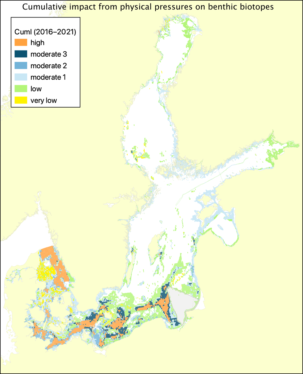
Combining the magnitude of the pressure and biotope sensitivities to derive the impact, the map shown in Figure 1 represents the resulting potential cumulative impact from physical disturbance. The results indicate that parts of the southern Baltic Sea and the Kattegat are potentially exposed to high impacts but also impacts with a low level are widespread. The high levels predominate in the deeper, offshore parts of the sea (> 20 m water depth in the southern Baltic Sea) and are often associated with areas exposed to major fisheries activity. The shallower coastal waters are potentially less severely affected, especially as bottom trawling fishery and disposal of sediments are typically constrained to deeper waters.
In most of the northern parts of the Baltic Sea, extraction and disposal of sediments is the most severe pressure. Locally, e.g., in archipelago areas and especially in coastal fairways, erosion from shipping is an important pressure.
All MSFD broad scale habitats used in the evaluation are potentially affected (Figure 2). On this Baltic-wide scale, all habitats exceed the quality threshold (i.e., some part of all MSFD BHTs exceeds the boundary set between low and moderate, although in some instances only by a small fraction). In 10 of the 18 habitats most of the area is unaffected by physical pressures based on the provided data and relatively low resolution of habitat maps in the coastal region. The percentage with cumulative impact varies between less than 10 % (offshore circalittoral rock and biogenic reef) and over 80 % (infralittoral sand). In most habitat types a physical disturbance of low and moderate (mostly lowest moderate category of m1) is dominating while a high degree of disturbance is typically seen in a comparatively small part of the disturbed area.
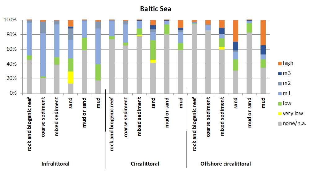
Figure 2: Evaluation results of the Cumulative impact from physical pressures on benthic biotopes in the Baltic Sea 2016–2021 (without loss). The graph shows the percentage of the individual MSFD broad scale habitat types potentially disturbed and the corresponding disturbance category (m1, m2 and m3 are three different grades of moderate disturbance, the category “none/n.a.” represents unaffected areas (none) including areas not evaluated (n.a.) due to lack of data; delivered data do not indicate areas with lack of data).
Breaking down the numbers for disturbance to the 17 HELCOM subbasins of the Baltic Sea (level 2 of the HELCOM assessment units), the results show regional differences in the extent of anthropogenic pressures and their expected impacts on the Baltic Sea and its seafloor (see Appendix A for details). The least amount of impact is predicted in the Bothnian Bay, the Gulf of Finland, the Bothnian Sea, the Northern Baltic Proper, the Quark and the Åland Sea. The remaining expected impacts mostly concentrate within the infralittoral zone (exceptions are the Gulf of Riga, Kattegat, Bay of Mecklenburg, Gdansk Basin, and Great Belt). The highest expected impacts are on the other hand seen in Kattegat, Great Belt, Kiel Bay and Bay of Mecklenburg. The highest expected impacts from the pressures used in this evaluation are predicted in the circalittoral zone, mainly due to bottom trawling fishery.
The following table shows the habitats for which none of the area exceeds the quality threshold in a specific subbasin (i.e., the quality threshold is achieved):
| Sub basin | habitats meeting the quality threshold in their respective subbasin (all others exceed the threshold): | |||
| Åland Sea | Offshore circalittoral mud or Offshore circalittoral sand | Offshore circalittoral rock and biogenic reef | Offshore circalittoral mixed sediment | |
| Bothnian Sea | all Offshore habitats | |||
| Eastern Gotland Basin | Offshore circalittoral rock and biogenic reef | |||
| Gulf of Finland | Offshore circalittoral coarse sediment | Offshore circalittoral sand | ||
| Northern Baltic Proper | Offshore circalittoral coarse sediment | Offshore circalittoral mud | Offshore circalittoral rock and biogenic reef | Offshore circalittoral sand |
| Western Gotland Basin | all Offshore habitats | |||
Note: some MSFD BHTs are identified as ‘mud or sand’ in the EUSeaMap 2021 classification due to uncertainties in the underlying sediment and geological information currently available. Future developments should improve the modelling and BHT mapping. A map showing the EUSeaMap 2021 MSFD BHT classification is provided side by side with the CumI evaluation for ease of comparison in Appendix J.
4.2 Trends
For this current evaluation, the determination and analysis of trends is not possible as the HOLAS 3 CumI evaluation is the first one that was done. However, before this evaluation, a number of test cases were performed and a Baltic-wide test run of the CumI with the HELCOM data from 2011–2016. These data are the ones that have been used for HOLAS II. The test cases are documented in the Appendix (B and C).
The Baltic-wide test run is only partly comparable to the current evaluation, especially since the underlying biotope map is a different one. For the dataset 2011–2016, the evaluation was based on the HELCOM habitats used for HOLAS II. The current evaluation (years 2016–2021) uses the EUSeaMap from 2021. Still, some similarities and trends can be identified (Figure 3). The most marked difference is a reduced magnitude of pressure for bottom trawling. As this is the most pronounced pressure especially in the Southern and Western Baltic Sea, a reduction in fishing intensity will immediately be visible in the end result. While the reduction in the Kattegat area is not visible at this scale, it can be seen in the Western and Southern Baltic Sea. The highly impacted area (orange colour) is smaller in the current evaluation especially in the Southern Baltic Sea around Bornholm and along the German/Polish/Lithuanian coast. In general, the low category (green colour) is more widely represented in the HOLAS 3 evaluation, with these low impact areas often replacing areas of higher impact categories in the earlier test case.
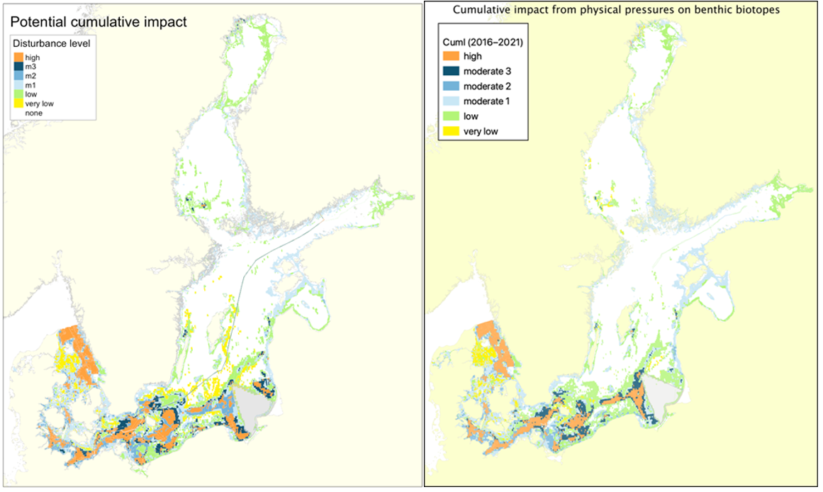
Figure 3: Overall comparison of the CumI test run (left) with the HOLAS 3 result (right). Despite a reduced comparability (see the text for this section) it is visible that the potential cumulative impact has decreased in some parts of the Baltic Sea, mainly due to a reduced fishing pressure in the Southern Baltic.
For a comparison of the impacts per habitat type, the new results were aggregated so that the offshore and circalittoral habitats of the same type were merged into the circalittoral alone. This corresponds closer to the HELCOM biotopes used in the test runs (Figure 4). The comparison shows the same pattern as the map where the “high impact” category is smaller with the recent data (2016–2021) especially in the Southern Baltic Sea, mainly due to the decreased magnitude of the bottom trawling pressure.
The mainly affected infralittoral biotope is infralittoral sand which also has the largest fraction with a very low impact. The fraction of infralittoral mud being affected seems to have increased, especially in the low impact category. The general pattern in the circalittoral biotopes is similar in both periods but the high impact category has decreased in the new evaluation. The smallest fraction of impacted area in the circalittoral is within the circalittoral mud and sand biotopes.
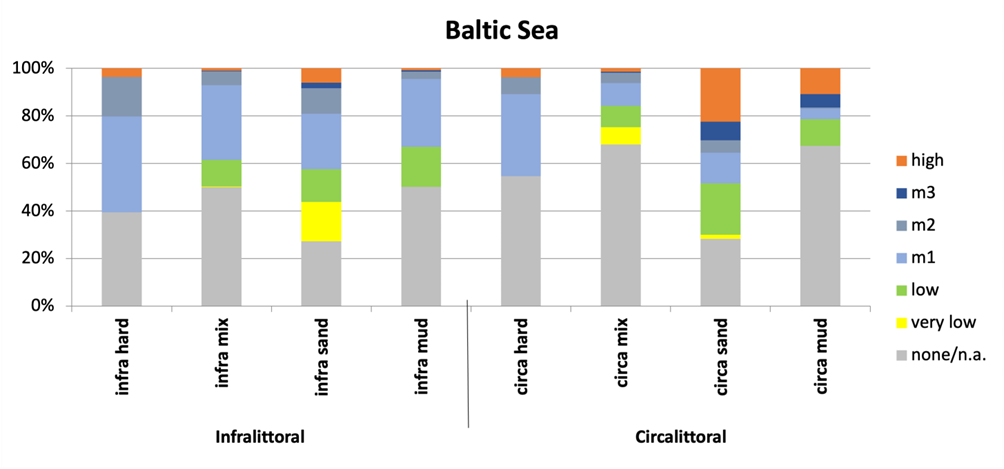
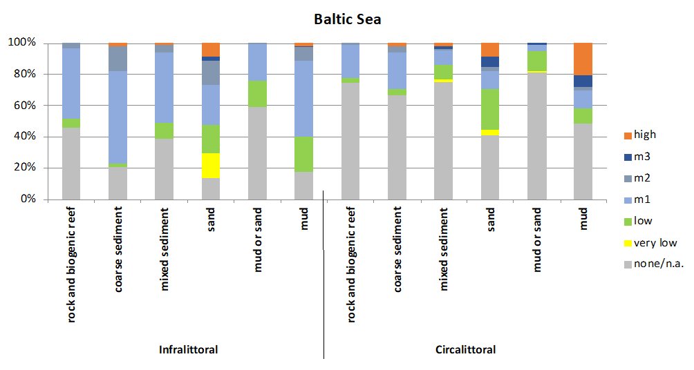
Figure 4: Evaluation results of the Cumulative impact from physical pressures on benthic biotopes in the Baltic Sea: upper panel: test run with 2011–2016 data and HELCOM biotope types; lower panel: HOLAS 3 result with 2016–2021 data when merging the circalittoral and offshore circalittoral categories into one category. Note: due to the changed biotope map (HELCOM biotopes in 2011–2016 and MSFD biotopes in 2016–2021) the comparison of results is of limited use.
4.3 Discussion text
A full discussion of the changes between assessment periods cannot be well defined due to the different base data underlying the evaluation. It would not be possible to properly distinguish between changes in these data and changes in the magnitude of the pressures. There is, however, some clear information of interest here which may be informative of general trends. Sand, for example, appears in the current and earlier test evaluation to be most heavily influenced by potential impacts from physical pressures (see Figure 4, above)..
In the current evaluation sand encounters the highest potential impacts within each of the three zones (circalittoral, infralittoral, and offshore circalittoral), followed by mud in all three zones. The next respective highest potential impacts for each zone are coarse sediments, except for the offshore circalittoral where it was mixed sediments (see Figure 2, above).
The apparent change between the current and test evaluations, despite the previously described comparability issues, does indicate the value of indicators such as the CumI. The apparent shift, broadly characterised by a move towards lower potential impact categories, appears linked to a change in physical pressures from fisheries activities. This is likely a combination of fisheries activities regulation and decrease of biomass of target species, e.g., cod. Specifically, reasons may be closures in certain areas during the assessment period. This emphasizes the fact that the spatial coverage of fisheries activities is a significant player influencing both the area covered and ultimately the outcome of the evaluation (as similarly shown where no fisheries activity data is available, i.e., in the Kaliningrad area (see Figure 1). The results also highlight the potential for such indicators in developing and evaluating future scenarios and thereby supporting management and measure setting. Low confidence could be expected in coastal areas where the low resolution of EUSeaMap is not reflecting the variation of habitats in the coastal areas. Furthermore, the EUSeaMap is not clear separating mud from sand in offshore and coastal areas, which might decrease confidence of the underlying habitat map.
There is always uncertainty in scientific data and evaluation methods which are based on natural phenomena and rely on a large amount of specific information. The CumI evaluation is being done in good faith to make best use of the available data, across the entire region of the Baltic Sea. The data used here are the ones Contracting Parties have submitted for the HELCOM HOLAS 3 process and have as such undergone review and quality control by member states and HELCOM. As well as issues related to the classification and resolution of human activities and the lack of well-established and harmonised data flows in HELCOM for human activities (in this instance related to loss or disturbance of the seafloor) the quality of seafloor habitat mapping (both nationally and currently available under the EUSeaMap 2021) has implications for the application of this indicator and thus influences the confidence.
Uncertainty evaluation method
As this text only evaluates pressure data, for the area for which pressure data are present, the confidence of the evaluation is rated according to the following categories:
- data quality
- temporal data coverage
- spatial data coverage
The rating is documented per evaluated pressure in the final GIS data set together with the impact evaluation. The rating is formatted as a string in the format ‘dxtxsx’ where the letters d, t and s represent the three categories (data quality, temporal coverage and spatial coverage) and the ‘x’ stands for the numbers within the categories as defined below.
When a pressure does occur in a particular area but information is missing in order to assess it, the string will be ‘d0t0s0’. This is the only case where all three categories are rated 0.
When no data or information is present for a particular area and thus the magnitude of the pressure or the resulting impact cannot be determined, the string ‘none’ is used for the confidence.
With this notation, we can distinguish between the following situations:
| Data | Pressure | Impact | Confidence | Remark |
| Present | Present | Yes | ‘dxtxsx’ | Impact is ‘very low’, ‘low’ and so on until ‘high’ |
| Present | Not present | ‘none’ | ‘dxtxsx’ | When it is known from the data that the pressure does not occur |
| Not present | Present | ‘none’ | ‘d0t0s0’ | Case of missing information for a pressure known to occur |
| Not present | Not present | ‘none’ | ‘none’ | When it is known that the pressure does not occur |
Currently, no method has been decided for an aggregation of the pressure-specific ratings to an overall confidence score for the whole evaluation. Nevertheless, the specific uncertainty values for the individually evaluated areas will be utilised in the integrated assessment of benthic habitats.
Thus, for example, ‘d2t3s1’ means: data present, quantitative and based on model, 5–6 years are covered within the assessment period of 6 years and data are present for this particular polygon.
This process supports the evaluation of that accompanying confidence evaluation, highlighting future required improvements (e.g., in data flows, monitoring or methodologies) but does in itself not adjust the outcomes based on the data quality.
Data quality
This rating gives information about the nature of the supplied data. The higher the quality of the data and the more information is present in the data, the higher the rating will be. Data can be based on a model, meaning that the applied buffer model in CumI relies on some general considerations on the extent and magnitude of the various Magnitude of Pressure (MOP) zones without being backed up by concrete data. Currently, only the bottom trawling data use real measurements to determine where the MOP zones are located:
0. No spatial data present (per pressure and country), only assumptions
1. Data present and qualitative
2. Data present, qualitative and based on model
3. Qualitative data based on real measurements
Temporal coverage
All pressure data are supposed to cover the whole assessment period of six years. When a year or more is missing in the data set or no information on the temporal distribution of the pressure is available, the rating is lower:
0. No information available on temporal coverage
1. 1-2 years are covered within the assessment period of 6 years
2. 3-4 years
3. 5-6 years
Spatial coverage
When a specific region or country does not report data and it is known that the pressure occurs in that area, this information can be documented here. It can be rated per pressure polygon but is typically used country-wide:
0. No data present
1. Data present
Possible future enhancements for uncertainty evaluation
Future evaluations should be based on a more rigid approach to assess the uncertainty. Ideally, all pressure data should already be delivered with an uncertainty score, e.g., for the pressure intensity or spatial extent. This rating should be performed by the member states and the uncertainty score be delivered via the data call and would ideally results in a numeric value (e.g., in terms of the standard error). Then, this uncertainty score can be propagated through the steps of the evaluation together with the data themselves. This will lead to an uncertainty evaluation that is at least semi-quantitative when using categories for the uncertainty, such as low, moderate, high or fully quantitative when using numerical values.
Current uncertainty evaluation results
Following the method outlined above, for the HOLAS 3 data the evaluation resulted in the following scores:
Bottom trawling fishery
The confidence is rated as ‘d3t3s1’ for all countries except Russia which is rated ‘d0t0s0’ due to missing data:
– data quality is rated 3 as values are based on reported measurements
– temporal coverage is rated 3 (no year missing)
– spatial coverage is rated 0 for Russia (assumed from how the data look like) and 1 otherwise
Mariculture
The confidence is rated ‘d2t3s1’ for finfish mariculture:
– data quality is rated 2 as data are used without the available quantitative information
– temporal coverage is rated 3 (one year missing)
– spatial coverage is rated 1 (assumed, as data set does not include information on reporting countries)
The confidence is rated ‘d2t0s1’ for Denmark and ‘d0t0s0’ for Germany for shellfish mariculture:
– data quality is rated 2 for Denmark as data carries no quantitative information
– temporal coverage is rated 0 (no information available for individual years)
– spatial coverage is rated 1 for Denmark, 0 for Germany
Extraction and disposal of sediments
Extraction of sand and gravel: the confidence is rated ‘d1t1s1’ for Estonia, Finland and Germany and ‘d0t0s0’ for the other countries:
– data quality is rated 1 as the reported extraction amount alone cannot be used (missing information on extraction depth and aerial extent within the extraction site)
– temporal coverage is rated 1 (we can exclude sites which have not been used within the assessment period)
– spatial coverage is rated 1 for Estonia, Finland and Germany, 0 for the remaining countries
Deposit of dredged material (areas): The confidence is rated ‘d1t3s1’:
– data quality is rated 1 as the reported deposition amount alone cannot be used (missing information on deposition height and areal extent within the deposition site)
– temporal coverage is rated 3 (data from 2021 are missing)
– spatial coverage is rated 1 (all countries have provided data)
Deposit of dredged material (points): The confidence is rated ‘d1t3s1’:
– data quality is rated 1 as the reported deposition amount alone cannot be used (missing information on deposition height and areal extent within the deposition site)
– temporal coverage is rated 3 (data from 2021 are missing)
– spatial coverage is rated 1 (all countries have provided data)
Germany and Sweden also have provided line data for deposits: The confidence is rated ‘d1t0s1’:
– data quality is rated 1 as the reported deposition amount alone cannot be used (missing information on deposition height and areal extent within the deposition site)
– temporal coverage is rated 0 (the data is assumed to only cover one-time events and no information is given for the other assessment years)
– spatial coverage is rated 1 (assumed that all countries have provided data)
Maintenance dredging (areas): The confidence is rated ‘d1t0s1’:
– data quality is rated 1 as the reported dredging amount alone cannot be used (missing information on dredging depth and areal extent within the dredging site)
– temporal coverage is rated 0 (as temporal information is not yet used)
– spatial coverage is rated 1 (assumed that all countries have provided data)
Maintenance dredging (points): The confidence is rated ‘d1t0s1’:
– data quality is rated 1 as the reported dredging amount alone cannot be used (missing information on dredging depth and areal extent within the dredging site) and most sites do no report the amount
– temporal coverage is rated 0 (as temporal information is not yet used and mostly not available)
– spatial coverage is rated 1 (assumed that all countries have provided data)
Dredging data from German (line data): no amount reported, maintenance dredging assumed, the confidence is rated ‘d1t0s1’:
– data quality is rated 1 as the dredging amount is not reported
– temporal coverage is rated 0 (as temporal information is not yet used)
– spatial coverage is rated 1 (assumed that all countries have provided data)
Pipelines and cables
Pipeline polygon data: The confidence is rated ‘d1t0s1’:
– data quality is rated 1 as there are no quantitative data on trenches and amounts
– temporal coverage is rated 0 (as temporal information is not yet used)
– spatial coverage is rated 1 (assumed that all countries have provided data)
Cables in operation: The confidence is rated ‘d1t0s1’:
– data quality is rated 1 as there are no quantitative data
– temporal coverage is rated 0 (as temporal information is not yet used)
– spatial coverage is rated 1 (assumed that all countries have provided data)
Platforms and wind farms
Wind farms in operation: The confidence is rated ‘d1t0s1’:
– data quality is rated 1 as there are no quantitative data
– temporal coverage is rated 0 (as temporal information is not yet used)
– spatial coverage is rated 1 (assumed that all countries have provided data)
Coastal protection
The confidence is rated ‘d1t0s1’:
– data quality is rated 1 as there are no quantitative data
– temporal coverage is rated 0 (as temporal information is not yet used)
– spatial coverage is rated 1 (assumed that all countries have provided data)
Shipping
The confidence is rated ‘d3t3s1’:
– data quality is rated 3 as there are quantitative measured data
– temporal coverage is rated 3 (as temporal information is not yet used)
– spatial coverage is rated 1 (assumed that all countries have provided data)
HELCOM completed a Red List assessment for Baltic Sea benthic biotopes, habitats and biotope complexes in 2013. For those benthic biotopes that had experienced, or were expected to experience in the future, a decline high enough to warrant a listing in the threat categories, were further considered to identify the major cause of decline. The threats were categorized and the main threat categories causing physical disturbance to benthic biotopes, based on used data, were ‘Fishing’, ‘Construction’ and ‘Mining and quarrying’, additional ones that may cause physical damage included ‘Tourism’, ‘Water traffic’ and ‘Ditching’ (HELCOM 2013a)’.
In the 2018 HOLAS II update of the ’State of the Baltic Sea’ report the top human activities causing cumulative impacts on benthic habitats were bottom trawling, shipping, recreational boating and sediment dispersal caused by various construction and dredging activities and deposit of dredged sediment (HELCOM 2018E). Based on the data available for the evaluation of the HOLAS II update, less than 1 % of the Baltic Sea seabed is potentially lost due to human activities while roughly 40 % of the seabed area was potentially disturbed during the assessment period from 2011–2016 (HELCOM, 2018E). However, the estimation does not reflect whether these areas are associated with adverse effects to the benthic biotopes, since the intensity of disturbance is unknown in the BSII assessment.
This HELCOM Cumulative impact from physical pressures on benthic biotopes indicator is structured around these main uses and human activities known to have impact on benthic biotopes through physical disturbance, especially those with large spatial impacts (e.g., impacting on a sub-regional or WFD water body scale). The “Themes” according to Table 2 Annex III in 2017/845/EU can be regarded as sectors (or drivers) of human activities. Following the DAPSI(W)R(M) framework (Elliott et al. 2017) the drivers (D) lead to actual human activities (A). These have been identified and are connected to the use categories. From these, the major physical pressures (P) were identified that will subsequently emerge. Every pressure is assigned to apply to either the habitat or biotope level (or both). These will cumulatively be responsible for major parts of the impacts on benthic biotopes on the regional scale. Table 3 summarizes the relationships of use categories, human activities (called “pressure” in the CumI evaluation and in this document) and the subsequent primary pressures on a larger scale affecting the marine environment.
Table 3: Primary pressures considered in the indicator and their relation to human activities and target components.
| Use category | Human activity | Primary pressures | Target components |
| Physical restructuring of rivers, coastline or seabed | Restructuring of seabed morphology incl. dredging and disposal of dredged matter | Suspended sediments | Habitat & species |
| Sedimentation, smothering | Habitat & species | ||
| Coastal defence and flood protection structures | Habitat loss, additional disturbance pressures during construction | Habitat & species | |
| Production of energy | Renewable energy generation including infrastructure | Habitat loss, additional disturbance pressures during construction | Habitat & species |
| Transmission of electricity and communication (cables) | Habitat loss, additional disturbance pressures during construction | Habitat & species | |
| Transport | Transport infrastructure | Habitat loss, additional disturbance pressures during construction | Habitat & species |
| Shipping | Abrasion | Habitat & species | |
| Suspended sediments | Habitat & species | ||
| Extraction of non-living resources | Extraction of minerals | Habitat loss/disturbance | Habitat & species |
| Siltation | Habitat & species | ||
| Extraction of living resources | Fish and shellfish harvesting (professional, recreational) | Abrasion | Habitat & species |
| Extraction of organisms | Species |
Other pressures not mentioned in Table 3 but important on a more local scale are here called secondary pressures. These come from various human activities and can be used in addition to the primary pressures if they are of importance in a specific spatial assessment unit or harmonised data collection can be achieved. As an example, tourism and leisure activities and infrastructure and their subsequent pressures can be regarded as secondary pressures, since they are local and therefore will typically not contribute significantly to the impact on the larger subbasin scale while they still might be important on a WFD water body scale or related to coastal habitats. This report only deals in detail with the primary pressures. The handling of secondary pressure, however, should follow the same principles as outlined here for the primary ones and they can be easily added in the calculation procedure.
In summary, all these activities leading to the mentioned pressures are showing a strong link to the MSFD and can be mapped to the corresponding pressures from the MSFD Annex III (Table 4).
Table 4: Brief summary of relevant pressures and activities with relevance to the CumI indicator.
| | General | MSFD Annex III, Table 2a |
| Strong link | Physical disturbance of the seafloor:
|
Physical
Biological
|
| Weak link |
Climate change effects on the Baltic Sea such as the rise of water temperature, change of sea levels and decrease of the ice cover will affect ecosystems and biota. Especially when benthic species exist at the edge of their distributional range (not uncommon in the Baltic Sea due to e.g., a strong salinity gradient), small changes in temperature and salinity can impact their abundance, biomass, and spatial distribution.
To address possible impacts of climate change on the functioning and outcomes on the indicator Cumulative impact from physical pressures on benthic biotopes, the HELCOM Climate Change Fact Sheet (HELCOM 2021b) was used to review environmental/ecological parameters that are affected by climate change and are directly linked to benthic habitats/biotopes (HELCOM 2021b, Fig. 2).
Although climate change might influence human activities such as fisheries and shipping (HELCOM 2021b, Fig. 2) which are addressed in the CumI as physical pressures, the focus here is on physiochemical parameters and their predicted changes potentially influencing biotope sensitivities. Generally, if a parameter negatively affects the sensitivity of organisms, the associated benthic biotopes might also become more sensitive towards this parameter or another pressures. As a result, the magnitude of impact from physical pressures will be higher (compare results in chapter 4). The following physiochemical parameters are directly affected by climate change and can influence the sensitivity of benthic biotopes by changing the sensitivity of their associated species (higher sensitivity is marked in bold fond, whereas reduced sensitivity is marked in underlined fond).
The sea surface temperature of the Baltic Sea has increased more than the average for the global ocean and will continue to rise everywhere in the Baltic and in all seasons. Vertical summer stratification will increase due to warming. Benthic species with a low thermal tolerance and living above the thermocline are more sensitive to warming temperatures. As a result, biotopes above the thermocline potentially become more sensitive.
The sea ice cover is expected to decrease. The ice season will become shorter and the maximum ice extent will decrease (Bothnian Bay, Bothnian Sea, Gulf of Finland, Gulf of Riga). This implies that photic periods of formerly ice covered infralittoral biotopes will extend, thereby potentially increasing benthic productivity. This might lead to increased resilience and a reduced biotope sensitivity.
Salinity and saltwater inflows. Salinity affects the dynamics of ocean currents and ecosystem functioning. Salinity decreases gradually from Kattegat to the Bothnian Bay. Inflows from the North Sea sporadically renew the deep water with saline, oxygen rich water. Overall, no statistically significant trends in salinity have been found and uncertainties of future projections are high. However, most simulations suggest that precipitation and river discharge will increase in the northern Baltic Sea region (Bothnian Bay and Bothnian Sea). Increased freshwater influx might cause salinity fluctuations, affecting species reproduction and survival, thereby increasing organisms’ sensitivity in coastal ecosystems. As a consequence, coastal infralittoral biotopes might become more sensitive.
The carbonate system regulates seawater pH. The amount of CO2 in the Baltic Sea surface water changes mostly due to biologically driven processes (photosynthesis and respiration), which induces seawater pH oscillations. In the long term, atmospheric CO2 increase will raise seawater CO2 concentration and cause pH decrease (ocean acidification). Over the long run species become less successful to build protective carbonate structures (such as shells) at lower pH. By reducing species’ resistance and resilience towards physical pressures, benthic biotopes potentially become more sensitive.
The mean sea level in the Baltic Sea responds to global sea level rise and regional land uplift. Baltic sea level is rising and will continue to rise. As a result, the current photic zones of benthic biotopes might decrease, resulting in a limitation of benthic flora and potentially reducing benthic productivity in infralittoral biotopes. In habitats where macrofauna is considered, sensitivity of infralittoral benthic biotopes might increase.
The wave climate in the Baltic Sea strongly depends on the wind field and shows large long-term variability. For the northern and eastern parts of the Baltic (Bothnian Sea, Gulf of Finland) a slight increase is significant and extreme wave height is projected. Greater shear stress increases the magnitude of physical pressure which is exerted on coastal benthic biotopes. Waves potentially homogenize the water column fully in some shallow water regions or partly in deep water regions, thus aerating formerly stratified waters. Increased oxygen concentrations can reduce organisms’ sensitivity and subsequently lower biotope’s sensitivity.
The following ecosystem parameters are indirectly affected by climate change and can influence the sensitivity of benthic biotopes.
The Oxygen availability is directly controlled by physical transport (air-sea exchange, advection and diffusion), water temperature and biological processes such as photosynthesis and demand for oxidation by remineralization of organic matter. Bottom water oxygen deficiency observed in a larger area of the Baltic Sea is a consequence of water column stratification and eutrophication. Projected warming may enhance oxygen depletion in the Baltic Sea by reducing air-sea and vertical transports of oxygen and by reinforcing eutrophication through intensifying internal nutrient cycling. However, the future development of deep-water oxygen conditions (i.e., in the Baltic Proper) will mainly depend on the nutrient load scenario. If nutrient loads are high, the impact of warming will be considerable and negative; if low, the effect will be small. Reduced oxygen concentrations can increase organisms’ sensitivity and the overall biotopes’ sensitivity. For consideration of oxygen depletion within the indicator evaluation see section 8.
The Nutrient concentration and eutrophication. Nitrogen and phosphorus pools are controlled by loads from land and atmosphere and influenced by oxygen-sensitive biogeochemical processes. Future load changes will have a stronger influence on nutrients than climate change, even though projected warming will increase nutrient cycling and reduce bottom water oxygenation. The riverine nutrient load is directly linked to the river run-off. Projections suggest that river discharge will increase in the northern Baltic Sea region (Bothnian Bay, Bothnian Sea). Increased freshwater discharge would bring more dissolved organic carbon to the sea, affecting benthic habitats by decreasing pelagic primary production and phytoplankton sedimentation (HELCOM 2021b, impact map).
Projected regional changes for some of the most relevant parameters in six particular subbasins of the Baltic Sea were taken from the impact map of the Climate Change Fact Sheet of the Baltic Sea (HELCOM 2021b). Potential impacts of the parameters on the outcomes of the indicator evaluation are addressed below. Please note that details of how a parameter’s impact can be implemented in layers of biotopes’ sensitivity are not discussed. The presented parameters have 1) direct societal relevance/experience and/or relevance for other parameters, 2) medium to high confidence of the changes relative to the noise and model/expert judgement uncertainty under the RCP4.5 scenario, and 3) a hotspot sub-region in the Baltic with medium to high confidence of patterns of the regional changes.
Baltic Sea entrance area (Kattegat, Great Belt, the Sound, Kiel Bay, Bay of Mecklenburg and Arkona Basin)
- Sea surface temperature would rise => increased sensitivity of benthic biotopes above the thermocline
- Mean sea level is projected to rise relative to the land => reduced benthic production caused by light limitation => increased sensitivity of infralittoral benthic biotopes
- higher storm surges would occur => shear forces: increased magnitude of pressure on coastal benthic biotopes => higher sensitivity of benthic biotopes in coastal areas; aeration in deep water regions => reduced sensitivity of benthic biotopes
- Higher atmospheric pCO2 increase seawater acidification => increased sensitivity of benthic biotopes
Every single parameter as well as the sum of all parameters result in a higher magnitude of impact of physical pressures on the benthic biotopes above the thermocline. This leads to a higher risk for a change in the environmental state.
On the contrary, storm surge driven aeration of the water column might result in a lower biotope sensitivity, leading to a reduced (magnitude of) impact of physical pressures on benthic biotopes in lower layers of stratified waters. The risk for a change in the environmental state might be reduced.
Baltic Proper (Northern Baltic Proper, Western Gotland Basin, Eastern Gotland Basin, Bornholm Basin and Gdansk Basin)
- Sea surface temperature would rise => increased sensitivity of benthic biotopes above the thermocline
- If BSAP measures on nutrient loads were to be implemented, phosphorus concentrations and algal blooms would decrease, and oxygen conditions of the deep water would improve => decreased sensitivity of benthic biotopes below the halocline
- Without load reductions, only minor changes in nutrient concentrations are expected => no effect on benthic biotope sensitivity is expected
- The combined effects of warming and planned nutrient reductions will eventually lead to less carbon reaching the seafloor, reducing benthic animal biomass.
- In shallow archipelago waters, the fates of benthic animal and plant populations depend on local variations in biogeochemistry and primary productivity => effect on biotope sensitivity can vary, but effect of rise in sea surface temperature on benthic biotope sensitivity is still present
- In the southern Baltic, mean sea level would rise relative to the land => reduced benthic production caused by light limitation => increased sensitivity of infralittoral benthic biotopes
- higher storm surges would occur => shear forces: increased magnitude of pressure on coastal benthic biotopes; aeration in deep water regions => reduced sensitivity of benthic biotopes
All parameters affecting infralittoral and circalittoral benthic biotopes above the thermocline result in a higher magnitude of impact of physical pressures on the benthic biotopes, thus leading to a higher risk for a change in the environmental state.
Storm surge driven aeration of the water column might result in a lower biotope sensitivity and hence a lower (magnitude of) impact of physical pressures on the benthic biotopes in lower layers of stratified waters. This effect might reduce the risk for a change in the environmental state.
Implemented measures on nutrient loads improve oxygen conditions of the deep water and result in a lower magnitude of impact of physical pressures on the (offshore circalittoral) benthic biotopes, thus leading to a lower risk for a change in the environmental state.
Gulf of Riga
- Sea surface temperature would rise => increased sensitivity of benthic biotopes above the thermocline
- mean sea level would rise relative to the land => reduced benthic production caused by light limitation => increased sensitivity of infralittoral benthic biotopes
- sea ice cover would decline => reduced sensitivity of infralittoral benthic biotopes
- higher storm surges would occur => shear forces: increased magnitude of pressure on coastal benthic biotopes; aeration in deep water regions => reduced sensitivity of benthic biotopes
Most parameters (except sea ice cover) affecting infralittoral and circalittoral benthic biotopes above the thermocline potentially result in a higher magnitude of impact of physical pressures on the benthic biotopes. However, the weighing of the listed parameters is unknown and no trend of the overall effect on the risk for a change in the environmental state can be given.
Aeration of the water column caused by storm surges might result in a lower biotope sensitivity and hence reduce the (magnitude of) impact of physical pressures on the benthic biotopes in lower layers of stratified waters. This effect might diminish the risk for a change in the environmental state.
Gulf of Finland
- Sea surface temperature would rise => increased sensitivity of benthic biotopes above the thermocline.
- mean sea level would rise relative to the land => reduced benthic production caused by light limitation => increased sensitivity of infralittoral benthic biotopes.
- sea ice cover, ice thickness and the length of the ice season would decrease => reduced sensitivity of infralittoral benthic biotopes.
- Wave heights would increase, and higher storm surges would occur => shear forces: increased magnitude of pressure on coastal benthic biotopes; aeration in deep water regions => reduced sensitivity of benthic biotopes.
Most parameters (except sea ice cover) affecting infralittoral and circalittoral benthic biotopes above the thermocline potentially result in a higher magnitude of impact of physical pressures on the benthic biotopes. However, as the weighing of parameters is unknown the overall effect on the risk for a change in the environmental state cannot be evaluated.
Storm surge driven aeration of the water column might result in a lower biotope sensitivity and hence reduce the (magnitude of) impact of physical pressures on the benthic biotopes in lower layers of stratified waters. This effect might diminish the risk for a change in the environmental state.
Bothnian Sea (Bothnian Sea and Åland Sea)
- Rise of sea surface temperature would be most pronounced in summer season => increased sensitivity of benthic biotopes above the thermocline.
- Winter precipitation including high-intensity extremes would increase => sensitivity of benthic species existing at the edge of their distribution might become more sensitive => increased sensitivity of coastal benthic biotopes.
- Increased freshwater discharge would bring more dissolved organic carbon to the sea, affecting benthic habitats by decreasing pelagic primary production and phytoplankton sedimentation.
- decline in sea ice cover => reduced sensitivity of infralittoral benthic biotopes.
Most parameters (except sea ice cover) affecting infralittoral benthic biotopes result in a higher magnitude of impact of physical pressures on infralittoral benthic biotopes, thereby potentially leading to a higher risk for a change in the environmental state.
High sea surface temperatures in summer might result in oxygen limitation, increasing benthic biotopes’ sensitivity below the thermocline. This in turn might result in a higher (magnitude of) impact of physical pressures, potentially increasing the risk for a change in the environmental state.
Bothnian Bay (Bothnian Bay and the Quark)
- Sea surface temperature would rise => increased sensitivity of benthic biotopes above the thermocline.
- Winter precipitation including high-intensity extremes would increase => sensitivity of benthic species existing at the edge of their distribution might become more sensitive => increased sensitivity of coastal benthic biotopes.
- Increased freshwater discharge would bring more dissolved organic carbon to the sea, affecting benthic habitats by decreasing pelagic primary production and phytoplankton sedimentation.
- sea ice thickness and the length of the ice season would decrease => reduced sensitivity of infralittoral benthic biotopes.
- Land is rising faster than the projected sea level and the mean sea level would sink relative to land => reduced sensitivity of infralittoral benthic biotopes.
While parameters directly affecting coastal benthic biotopes potentially result in a higher (magnitude of) impact of physical pressures, parameters reducing light limitation (reduced ice cover and sea level drop) potentially lead to less sensitive benthic biotopes, resulting in lower (magnitude of) impact of physical pressures. However, the weighing of parameters is unknown and the risk for a change in the environmental state cannot be evaluated. Especially underlying habitat data needs to be improved and regionally harmonized in order to give more concrete management recommendation and to stop further deterioration of the status of the sea bottom.
The benthic biotopes in the Baltic Sea are negatively affected by several human activities causing physical disturbance to the seafloor, potentially leading to physical or functional loss of biotope areas. Using the HECOM core indicator Cumulative impact from physical pressures on benthic biotopes (CumI) it is possible to map the pressures spatially, perform a predictive evaluation of their cumulative (i.e., aggregated) potential impact and give a comprehensive uncertainty analysis. Especially the uncertainty evaluation reveals where both the data quality can be improved in future and the type of data that should ideally be delivered for future evaluations. It also shows how the indicator itself can be improved to utilize the full extent of the delivered data (e.g., an enhanced frequency evaluation; see below).
The current evaluation of the CumI includes bottom trawling fishery and mariculture, extraction and disposal of sediments (e. g. dredging and dumping), pipelines and cables, platforms and wind farms, coastal protection and shipping. The highest cumulative impact from the physical pressures listed here generally occurs in the southern part of the Baltic Sea and in the Kattegat, dominated by wide-area pressures such as bottom trawling fishery. Bottom trawling can have long-lasting effects on biotopes, especially those dominated by long-lived benthic fauna. Extraction and disposal of sediments is generally the most severe pressure in most of the northern areas of the Baltic Sea. Locally, in archipelago areas and especially in coastal fairways, erosion from shipping can have an impact on seafloor sediments. Pressures such as coastal protection are constrained to very narrow stretches or points on the coastline and are occurring in the whole Baltic Sea region. A static overview of these pressures, cumulated to predicted impact category, is available in Figure 1, and more detail can be achieved regarding placement and footprint via using the HELCOM Map and Data Service, MADS. In the current evaluation the Broad Habitat Type (BHT) of sand encounters the highest potential impacts within each of the three zones (circalittoral, infralittoral, and offshore circalittoral), followed by mud in all three zones.
It must be noted that the indicator does not perform a mapping of actual real impacts. It is based on a modelling approach, using biotope sensitivities (i.e., the sensitivities of the benthic communities living in specific broad habitat types) and the magnitude of the pressure. The resulting impacts can be interpreted as the potential change in the environmental state of benthic biotopes, given an undisturbed environment.
8.1 Future work or improvements needed
Human activities data
There is a clear need to improve the harmonisation and regular collection of relevant human activities data in the HELCOM region. Addressing this is considered as important not only for the CumI indicator but for a number of other relevant processes in HELCOM or future HOLAS assessments. It is important that such issues will be considered under the post-HOLAS 3 review process and the issue has already been raised to the State and Conservation Working Group. This also includes the reporting of human activities data with proper and uniform metadata (regardless of whether actual data are delivered too) making it possible to clearly distinguish between data not reported, not available or a pressure not being present.
Benthic habitat maps
The current quality
of benthic habitats maps can be a limiting factor in such assessments and improvements in both national and regional maps to support future assessments are vital.
Bottom trawling fishery
To assess the magnitude of trawling pressure, CumI uses/applies surface SAR which summarizes surface abrasion caused by all trawling activities within a defined space and time. More detailed information on trawling gear types or métiers has now become available. Different trawling activities penetrate the seabed substrate to different extents and there is growing evidence that depletion of benthic fauna correlates with penetration depth (Hiddink et al. 2017). Consequently, penetration depth of the trawling gear types/métiers should be taken into account in addition to the SAR values to assess the magnitude of pressure caused by physical disturbance through mobile fishing gears (Eigaard et al. 2016, ICES 2016, Rijnsdorp et al. 2020).
In order to reduce pressure and impact on the seabed caused by bottom trawling, an ICES advice exploring management scenarios for the EU was recently released (ICES 2021). The following management options are not (fully) captured in the CumI. Explanations are given below along with suggestions for future improvements:
- Gear modification in terms of reduced penetration depth, resulting in lower catch rate
Penetration depth is not part of the SAR value and data on gear types or métiers are not available. Since penetration depth cannot be reflected in the current evaluation, this management option would have no effect on the CumI. The issue on penetration depth dependent depletion was discussed in the past and is hopefully part of the future development. In line with this thought, ICES (2019b) suggested an alternative to present abrasion pressure that takes account of both, the footprint (SAR) of the trawl pass and the depletion of the gear used, by summing up the product of SAR and for all different gear types used. This product would directly correlate with the magnitude of abrasion pressure by bottom contacting fisheries.
- The removal of fishing effort by particular individual métiers (métier prohibition).
In the Baltic south of Åland/Gotland bottom contacting fisheries is the dominating pressure. In this area the removal of an individual fishing métier will have an effect on the CumI (via a reduced SAR value), if a) the métier is the only one used in the trawled area and b) the prohibited métier is not replaced by another métier. The magnitude of the effect directly correlates with the size of the affected area within a single BHT. However, if fishing activities in a c-square consist of multiple métiers, the effect size caused by an individual métier prohibition will be lower. This management option can be detected by the CumI through a reduced SAR value. CumI’s sensitivity (to this management option) can be improved by more detailed spatial and temporal information regarding applied métiers as suggested under 1).
In addition, further improvements could also be achieved related to the spatial accuracy and frequency of certain pressures by including, or better utilizing, AIS data (Automatic Identification System) in future assessments.
Pressure frequency evaluation
When the CumI was developed for HOLAS 3, frequency information was not readily available for the individual pressures. Hence, frequency is currently not used in the evaluation. To keep the current evaluation as close as possible to the agreed evaluation protocol for HOLAS 3, frequency information now available in the newly submitted data sets is still left out.
In the agreed CumI method, frequency is determined on the basis of the number of pressure events per year. However, this kind of information seems to represent a rare case and was not given in the submitted data. Much more often, frequency has now been reported in terms of “in how many of the 6 assessment years did the pressure occur?”. For this kind of data, the frequency can be interpreted as:
- occasional = occurs in 1 (of 6) years
- regular = occurs in 2-3 years
- frequent = occurs in 4-5 years
- persistent = occurs in all 6 years
This approach could be implemented for the updated data sets and used in future HOLAS assessments.
Consideration of oxygen depletion
Biotopes that are frequently, but not permanently affected by oxygen depletion, have a higher sensitivity against further deterioration. These biotopes already are under a certain physiological stress and may even have been impacted already. In order to account for this, it must be known where the areas of temporary oxygen depletion are located. Within the HELCOM 2011–2016 assessment (HOLAS II 2018 version), a data layer was available on the oxygen status that is suitable for this purpose (published through the HELCOM Map and Data Service).
As a first approximation, such an area being regarded as sub-GES in terms of oxygen status could be used to decrease the underlying biotopes’ resistance by one class if it is not already classified as high. In a more differentiated approach, actual oxygen concentrations and the duration of phases with oxygen depletion could be used. Areas where the biotopes’ resistance is decreased could then be identified as the areas having oxygen concentrations in the bottom water layer of less than 2 mg/l more than once per year (the exact amount would need to be specified). Spatial modelling of oxygen concentrations would even allow to use a specific number of days with concentrations less than 2 mg/l.
It is important to note that areas with permanent hypoxia (or having a duration of several years) are not considered here. These biotopes will already have reacted to the oxygen situation in a way that has altered or even removed the original biotopes. In parts of the biotopes, oxygen depletion may even be the natural environmental characteristic. Changing the sensitivity of these biotopes will thus not reflect the already altered state.
Sensitivity scores and ground truthing
The approach applied in this indicator utilises sensitivity scores as part of the basis on which predicted impacts are derived. These sensitivity scores are based on expert judgement, literature, experience and, where required, expert evaluation. Sensitivities have been regionally reviewed and adapted where required for sub-regional specificity and are therefore considered to be of low confidence. However, as with all scientific endeavours knowledge increases and better information becomes available over time. New sensitivity scores should be included as they become available and designated scientific work on this issue is likely highly valuable to support the evaluation of benthic habitats. Likewise, studies to evaluate or ground truth the in-situ relationship between status of benthic habitats (and their biotopes) in relation to the expected impacts generated via CumI would be valuable.
The general concept of the CumI indicator follows the requirements of the EU commission decision 2017/848/EU. For the MSFD criterion D6C3, the decision requires to look at the extent of the area that is adversely affected by physical disturbance. This means, the CumI needs to assess the environmental impacts from those physical pressures and cannot be restricted to just mapping the actual magnitude of the pressure. The decision explicitly states in the description of MSFD criterion D6C3 that the assessment should include
“… change in its biotic and abiotic structure and its functions (e.g., through changes in species composition and their relative abundance, absence of particularly sensitive or fragile species or species providing a key function, size structure of species)”.
The mapping of the pressures themselves is the objective of the MSFD criteria D6C1 and D6C2. The wording of the decision makes it clear that the target of the criterion D6C3 is the
“… change in […] structure and […] function”.
It is not the state as such, in terms of its absolute position on a status scale (such as the GES scale). What the CumI calculates is rather the spatial extent of state changes that are to be considered adverse effects (in terms of a certain magnitude of the impacts).
These requirements make it necessary to perform a transformation of the abiotic pressure data to the level of possible environmental impacts (i.e., state changes) from these pressures on the biotopes and their biota. This is done by using the sensitivities of the biotopes (derived from sensitivities of the biotope’s species) on which the pressures occur. The sensitivity information is then combined with the magnitude of the pressure to derive the possible environmental effect.
The indicator concept follows the same principle as the OSPAR BH3 indicator Physical damage of predominant and special habitats. The OSPAR indicator is currently constrained to the pressures bottom trawling and aggregate extraction, while the HELCOM CumI indicator also includes other physical pressures.
The evaluation presented in this report, uses HELCOM data from HOLAS 3 as operated as closely as possible to agreed HELCOM procedures and methods of data collection and handling. Further, the framework conditions (buffer distances, categories of magnitudes of pressure, etc.) used by HELCOM in the HOLAS II assessment have been used in the present evaluation, as far as possible.
A German (see Appendix B) and Swedish case study (see Appendix C) are partly using deviating conditions from the ones presented in the main body of this report.
In general, the evaluation for the Cumulative impact from physical pressures on benthic biotopes is performed using a Geographical Information System (GIS) as both the data and consequently also the actual evaluation are spatial information in the form of vector data (point, polyline or polygon data). Raster data are converted to vector data for evaluation. The evaluation procedure is a transparent and in principle easily followed step-by-step approach, taking the various GIS layers that are the basis of the biological and pressure information and doing certain spatial ‘intersect’ and ‘union’ operations on them.
To facilitate the evaluation, an R script is provided, implementing the current CumI evaluation. It can be customized in various ways. The R script is available on the EN BENTHIC workspace (in the HELCOM portal) together with a documentation, the used data layers and the resulting evaluation results. The script is currently at version 2.3 (as of 2023-02-21). In addition, the CumI script is also available at GitHub under https://github.com/torstenberg/CumI. There, all versions are stored and versioned and it is possible to contribute to the further development, either by forking the script or by issuing pull requests.
The CumI evaluation can also be done using the commercial ESRI ArcGIS software (version 9 or higher), the free QGIS software or any other GIS software capable of handling vector data. For this, the processing steps documented in the R script need to be replicated.
9.1 Scale of assessment
The indicator can be used with all four defined spatial HELCOM assessment levels depending on the respective requirements of the assessment, e.g., HELCOM, MSFD or WFD. For this document, the CumI was calculated for the whole Baltic Sea (HELCOM marine area 2018), and the results were broken down to the 17 HELCOM subbasins which represent major ecologically relevant regions in the Baltic Sea (see Appendix A). The results can be divided further into the coastal and offshore divisions (HELCOM assessment level 3) and into the WFD water types or water bodies (HELCOM assessment level 4).
The assessment scale may also depend on the quality of the underlying input data and their spatial resolution. In order to achieve comparable results which can also be used across different indicators and descriptors, it is recommended that the evaluation should be based at least on the 17 HELCOM subbasins as defined in the HELCOM Monitoring and Assessment Strategy Annex 4.
In national applications, other appropriate spatial subdivisions can be used, depending on the use-case and the availability of more detailed data. For such applications, typically a much more detailed biotope map will be needed.
9.2 Methodology applied
The starting points of the evaluation are a biotope map and a range of pressure maps. In principle, the biotope map/layer is carrying sensitivity information for the individual biotopes and will be evaluated against each of the physical pressure layers (using the magnitude of pressure) separately (see Figure 5). These pressure layers contain data for physical disturbance and loss (areas with physical loss are removed from the CumI evaluation in the last step of the process). The result is a set of layers with potential impacts on the benthic biotopes originating from the individual pressures used in the evaluation, i.e., one layer for each of the pressures.
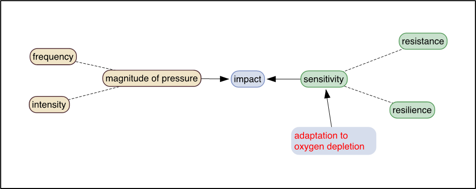
Figure 5: Overview of the evaluation protocol for a single pressure. The pressure is represented in terms of its magnitude of pressure and is combined with the sensitivities of the benthic biotopes.
The different impact layers are subsequently cumulated using a hierarchical approach in which pairs of impacts are combined using a cumulation matrix (Figure 6). The order of the pairing is arbitrary.
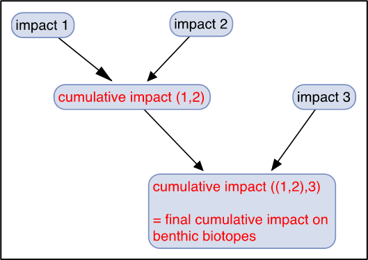
Figure 6: Process of cumulation using a pairwise spatial union process. In this example, three different impact layers are cumulated. Two of them (impact 1 & impact 2) are combined first. Next, the result of this union is an initial cumulative impact and is subsequently combined with impact 3. The result of this second union is the final cumulative impact on benthic biotopes.
Processing of pressure data
The individual pressures must be present as separate spatial data layers. The pressures should be quantified according to the magnitude of pressure, using the four classes very low, low, moderate and high. Areas without pressure should be marked as having a MOP of ‘none’. Also, areas without information should be tagged separately (e.g., with ‘unknown’). The magnitude of pressure is represented as a function of pressure frequency, intensity and range. The duration of individual events is currently not considered, as well as the general temporal aspects of pressures. The three elements of the magnitude of pressure are defined as follows:
- Frequency – the number of pressure events per time unit
- Intensity – the strength, concentration or power of the pressure
- Range – the exact size and extent of the polygons in the pressure layer
All these parameters vary in time and in space and make it a complex task to quantify the magnitude when it is applied to determine impacts on benthic biotopes. This is because a pressure is typically dynamically changing and the resulting impact on the biotopes is not a static status reached linearly after a pressure ceases. In every phase with a ceasing pressure, recovery of the organisms and their environment may take place and shift the starting level for the following pressure event. Also, the recovery process may not follow the same trajectory as the deterioration. It is impossible to reflect this complexity without dynamic modelling of all involved processes. Therefore, the indicator uses simplified methods.
There are various ways to reflect the intensity of a pressure within its range:
- Assignment of the whole range/area of the pressure to the same intensity, regardless of the distance to the source of the pressure. If there are more than one pressure source, the individual polygons in the pressure layer can have differing pressure intensities. This option is not used in the CumI method.
- Divide the range/area of the pressure into zones of different intensity. The zones typically have a decreasing intensity the further away from the pressure source they are located. Within each zone, the intensity is constant. This option is used for most of the pressures in the CumI method. A number of default zones (also called buffers) are defined in the CumI method. These are listed in Appendix D. These values of the pressure-specific sizes of the zones/buffers and their pressure intensities are a default setting. They should not be interpreted as fixed and unchangeable. When specific information on the nature of a pressure is available, especially based on actual data or national agreements with member states, those specific values should be used for the respective area of applicability instead of the default ones.
- Use pressure-specific continuous intensity values, based either on a spatial intensity function or algorithm, or based on actual measured or reported data. This option is used in the CumI method for intensity (and frequency) of bottom trawling fishery.
In order to be able to evaluate the magnitude of pressure against the respective sensitivity of the underlying benthic biotopes, the intensity must operate on the same scale throughout all pressures, i.e., a pressure intensity of e.g., “0.45” or “moderate” must have the same meaning in terms of the potential impact across the various pressures used. The pressure intensity for a given pressure layer must thus be translated to a common scale ranging from 0 to 1:
- Value of 0: no intensity = no pressure
- Value of 1: intensity leads to complete loss of function or loss of biotope (for the most tolerant biotope)
For each biotope, a specific intensity of each of the considered pressures will result in the loss of function (e.g., a pressure of sedimentation with a height of 1 m from the activity “Disposal of dredged matter”). In order to be comparable (i.e., operate on the same scale), the intensity of every pressure must thus be specified against the same biotope (i.e., against the same relative sensitivity).
The pressure frequency is independent of the biotope sensitivity and can be classified in absolute values for each pressure. It is divided into four categories:
- very low = occasional (less than once a year)
- low = regular (once per year)
- moderate = frequent (two to three times per year)
- high = persistent (more than three times per year or permanent)
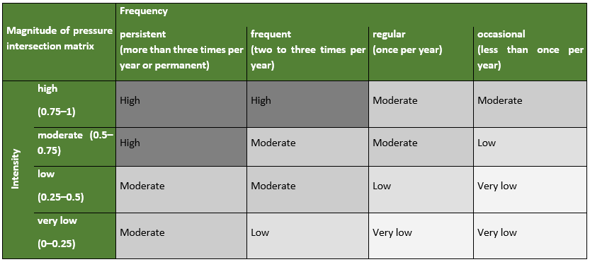
If both intensity and frequency carry a meaning for a certain pressure and data for this is present, the magnitude of pressure is derived from the following matrix (Table 5).
Table 5: Intersection matrix when combining pressure frequency and intensity into overall magnitude of pressure. The frequency categories are adapted from BioConsult (2013), the intensity scale pragmatically divided into four equidistant classes.
While some pressure data are available as numerical values that allow for the direct quantification of the intensity and frequency of the pressure, others might only be available in terms of presence data. For some pressure types, the concept of frequency is even not applicable. In order to use presence data for pressures, a quantification of these data using typical values found in literature or by empirical expert judgement is needed. For this purpose, the weighting factors for the Baltic Sea Pressure Index (BSPI: Korpinen et al. 2013) may be utilized in a modified way (not used in the current evaluation). Several of the data layers are only available as point data, e.g., giving the amount of dredged or disposed material in tonnes but without spatial extent, intensity or frequency. In order to use this kind of data, suitable values for those missing properties need to be found from literature or by expert judgement as was done in the HELCOM HOLAS II assessment for the BSII based on results from the expert survey and the literature survey. The spatial extent and intensity of the pressures may be adjusted based on detailed national data or technical information. This can be used to take into account local specifications that might otherwise be lost in a general Baltic-wide approach.
Current application: Only for bottom trawling fishery and shipping the pressure dataset was detailed enough to actually calculate and use specific spatial intensity values for the evaluation. For all other pressures, only the intensity was available or could be derived from the raw data, or the frequency of the pressure was irrelevant. In these cases, the intensity was directly used as the value for the magnitude of pressure without further use of the above intersection matrix. The following sections present in detail, how the pressure maps were implemented for the evaluation (also see the documentation in the R script).
The intersection process for impact determination
After the MOP of the pressures have been determined and the sensitivity against the pressures has been assigned per biotope type, the biotope sensitivity is combined with the magnitude of pressure for each pressure separately (Table 6). This results in one layer of potential impact per pressure. Since both sensitivity and magnitude of pressure are ordinal variables (i.e., categorical variables with a specific ordering) no meaningful arithmetical operations can be done with them. Just as the derivation of sensitivity of biotopes and magnitude of pressure themselves, the combination of these two must be done using a matrix. This matrix converts pressure into potential impact using biotope sensitivity (replacing the original weighting factors used by Korpinen et al. (2013)).
Unless the matrices for MOP and sensitivity, this intersection matrix is dividing the moderate class into three distinct classes (Table 6). This allows a refinement for the classification of severe disturbance. Note, that at this stage, no (functional) loss can occur. In the CumI, functional loss is only resulting from cumulation of two or more pressures, not from a single pressure. Loss at this stage is thus always direct physical loss from the respective MOP of the pressure. The classification, whether a single pressure is to be treated as loss, is done on an abstract level in the interpretation of the pressure (see Appendix D) and that classification only deals with physical loss according to the EU definition in 2017/848/EU.
Table 6: Intersection matrix to combine magnitude of pressure and biotope sensitivity to potential impact from physical pressures on the benthic biotopes with subclasses for resulting moderate impacts into three classes.
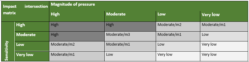
Further, all impacts above low, i.e., moderate (as m1, m2 or m3) and high are classified as significant impacts or adverse effects, respectively. The number of four classes for significant impacts is similar to OSPAR BH3 where five disturbance classes are used. However, nine disturbance categories are used in total for the BH3 evaluation in the North Sea in contrast to a total of six disturbance classes in the final cumulation step in the Baltic Sea.
Table 7: Classification of disturbance and loss according to the different impact categories in the evaluation procedure. The boundary between low and moderate is the boundary of significant impacts.
 The differentiation of the significant impacts moderate and high into 4 classes (instead of 2) enables a more precise allocation, in particular for the later separation of functional loss in the cumulation process.
The cumulation process
The cumulation process is the last step in the calculations of the indicator. This is done using a hierarchical approach. In order for the impact to cumulate, the effects of the pressures need to act on the same area and at the same time or at least within the recovery time of the biotope since the last pressure event (as described in Table 9). Overlap in space (area) will automatically be handled when spatially intersecting the impact layers. Overlap in time cannot be seen from the impact categories. For simplicity and to use a precautionary approach, it is assumed that all evaluated pressures do overlap when data from the same year or assessment period are used or when the pressure is not just occasional. This means, in the current evaluation no temporal aspect is included.
The following rules are applied for the cumulation process:
- The cumulative impact is determined using the instructions in Table 8 below
- If one of the resulting impacts is very high, it is considered a functional loss. The final cumulative impact is then also loss and need not be further cumulated
Table 8: Resulting cumulative impact when any two separate impacts are cumulatively intersected. The category very high is considered a functional loss.
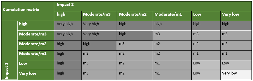 Note, that e.g., three separate impacts are cumulated by first intersecting two of them and then applying the matrix again with the cumulative class and the third impact class. As an example, the three different moderate impacts m1, m2 and m3 will always cumulate to high, regardless of the order the cumulation is applied in. The same is true for another example of the different impact classes low, m3 and m2, which will always cumulate to high, irrespective of whether the highest or lowest impact will be cumulated first (see Figure 7).
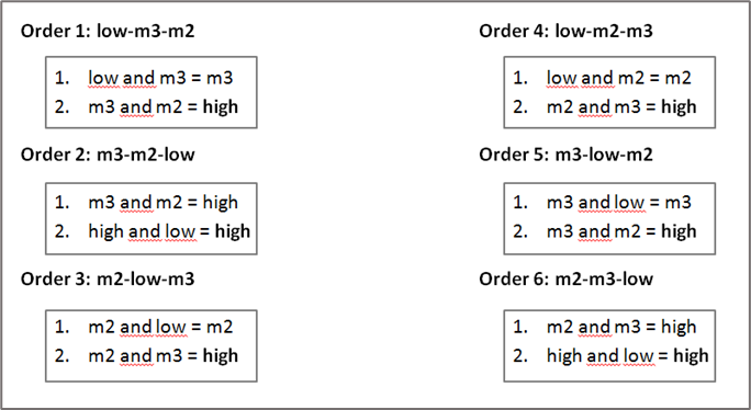
Figure 7: Example for the cumulation process using the cumulation matrix with all possible different orders of three impacts.
These cumulation rules are specified such, that low and very low impacts together do not escalate to the next higher impact class (sort of additive cumulation) since the assumption is that such impacts do not typically interfere with each other and produce multiplicative effects. Moderate impacts, however, may escalate to high or very high impact when cumulated, since these already are regarded as “significant” state changes and the risk of multiplicative (synergistic) effects is high. The higher class of two impacts determines the cumulation result at least to prevent averaging of impacts in the cumulation process. Antagonistic cumulation is regarded as not being a relevant option for this indicator where different pressure layers are evaluated.
Handling of physical and functional loss
The CumI handles both physical and functional loss in a special way. As loss is not part of MSFD criterion D6C3, the respective areas are not included in the CumI result.
Certain physical pressures may immediately lead to a physical loss of habitat. This is defined at pressure level and is part of the ongoing work in the EU technical group TG Seabed. This direct loss is not part of the actual CumI evaluation. The CumI only evaluates the areas where no direct loss occurs. This means that the areas indicating direct loss are removed from the pressure maps and stored separately.
Physical pressures may also lead to a functional loss by their cumulative impact when they act in combination by spatially and temporally overlapping each other and reaching a certain impact level together. Such pressures act on the biotopes at the same place and at the same time. When such a functional loss is detected during the evaluation procedure, the respective area is subsequently also moved from the CumI evaluation the separate map with loss, just as done for direct loss.
Both the direct and the functional loss are combined and can be provided as a separate map. This is one of the main parts of the information needed to assess MSFD criterion D6C4 (apart from other, non-physical anthropogenic pressures causing habitat loss).
Data format
All data layers need to be in vector format as georeferenced GIS layers. The CumI evaluation process works with polygon data. Point or polyline vector data is converted to polygons before entering the evaluation by buffering the features spatially in the GIS using various so-called “buffer models” (see Appendix D). In certain cases, also polygons are buffered spatially to accommodate for specific pressure settings. The process of buffering assigns certain pressure intensities to a specific zone around the point or polyline, depending on the distance from the source of the pressure. Raster data is converted to vector format before it can be used in the evaluation. This results in a vector layer with rectangular polygons.
Spatial resolution of data layers
Using vector data as much as possible enables the CumI to use the actual extent of the individual pressures without the need to generalise the data spatially (e.g., by translating the pressure data onto a uniform grid). This is the ideal case with respect to the spatial resolution. In the case of point or polyline data, the buffering process makes sure to approximate the real extent of the pressure as much as the information behind the data allow. Raster data should have a spatial resolution that is as high as possible.
Generally, the spatial resolution of the pressure data should correspond to the resolution of the biotope map used for evaluating the pressures. When the polygons in the pressure data are much larger than the biotopes due to a low spatial resolution of the underlying pressure data (i.e., the pressure data are either rough approximations or generalizations), the resulting evaluation will contain artifacts where impacts are predicted that are not possible in reality.
The biotope data
The basis of the evaluation is formed by a biotope map showing the biotope types occurring in the assessment area. The term “biotope” refers to the physical (abiotic) habitats including their associated biological benthos communities (Cochrane et al. 2010, Olenin & Ducrotoy 2006). For the MSFD Descriptor D6 (“Seafloor integrity”) of the EU Commission Decision 2017/848/EU, the term “habitat” is also to be interpreted as a biotope.
The biotope types on the map should not spatially overlap but always be adjacent to each other. If there is a need to define more than one biotope type per area, biotope complexes (e.g., as defined in HELCOM HUB) should be used instead. For subregional or national assessments, a detailed biotope map can be used that differs from the one used for HOLAS 3. The CumI method does not prescribe the use of a specific biotope map. Appendix B gives an example of a case study in German waters using a differentiated biotope map.
Current application
For the HOLAS 3 evaluation presented in this report, the EUSeaMap in the version of September 2021 has been used. As the Baltic part of the EUSeaMap does not include the Kattegat, part of the corresponding map for the European Atlantic and Arctic region was merged into the data (as long as it is within the HELCOM assessment area).
The biotope sensitivity information
Every biotope type in the map is ideally assigned to an individual sensitivity category (very low, low, moderate, high) against each of the considered pressures. If no pressure-specific sensitivity information is available, a general sensitivity against physical pressures as a whole can be used instead.
In principle, sensitivity is derived from its resilience and resistance towards the respective pressures. These two sensitivity components are defined as follows:
- Resistance – the ability to withstand and tolerate a pressure without a change of the (environmental) state of the biotope
- Resilience – the ability to recover from a pressure when it ceases. Here used in terms of the time needed to recover (recoverability or recovery time)
Both components of sensitivity are needed in order to capture the most important aspects of the reaction of species towards a pressure. For example, using resilience alone (in terms of recovery time which is often measured using longevity information) can result in a skewed evaluation. The most long-living species in the Baltic Sea is the Ocean Quahog Arctica islandica. It has a long lifespan, but this does not necessarily mean that the species is particularly sensitive in general. In fact, the species is quite resistant towards e.g., oxygen deficiency as one of the possible pressures resulting from extraction and disposal of sediments. When considering resistance along with resilience, the overall sensitivity is evaluated in a more realistic way.
When based on resilience and resistance data, the sensitivity of the biotope is determined using a sensitivity intersection matrix (Table 9):
Table 9: Intersection matrix when combining resilience (in terms of recovery time) and resistance towards physical pressures into the sensitivity of a benthic biotope. This matrix is adapted and modified from BioConsult (2013) in order to be compatible to other classifications e.g., used in the BSPI (HELCOM 2010) and by La Riviére (2016). The matrix also to a large degree corresponds to the one proposed by ICES (ICES 2016; WKFBI work).
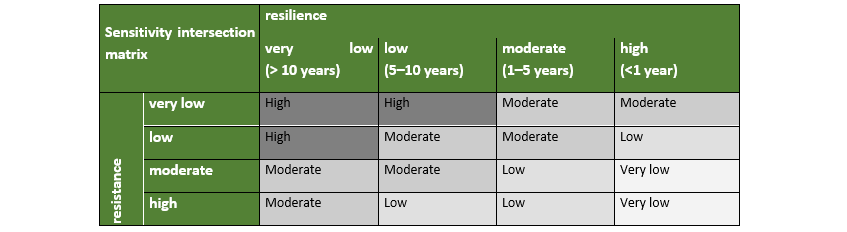 Alternatively, if there is no specific information available on resistance and resilience, an existing sensitivity score can be used which indirectly already takes resistance and resilience into account. Further, the sensitivity can vary spatially within each biotope type depending on environmental parameters such as salinity.
The use of the sensitivity in the evaluation implies that the sensitivity values should not reflect the state of a biotope after having been under pressure (i.e., the present state with potentially a reduced set of species or an altered hydromorphology) but rather some kind of modelled and static[2] sensitivity based on the potential set of species, habitats and biotopes which would naturally occur within the considered biotope types used for the evaluation. The reasoning for this is as follows:
The resilience depends on the ability of a species or individual to recover from a pressure. When a population has been killed, it needs to re-colonize the affected area. Thus, the time needed for this process (including reproduction and growth) is determining the resilience. This is independent from the intensity of the pressure (assuming the pressure has ceased) but can depend on the frequency of recurring pressure events when the events are more frequent than the time needed for recovery. So, when the frequency and intensity of the pressure increase, the highly sensitive species may drop out. The remaining community will have a higher resilience resulting in a lower biotope sensitivity. Frequently recurring pressure events would thus eventually lead to biotopes having a lower biotope sensitivity as only the most tolerant species would remain. Lower sensitivity would lead to a lower potential impact within the CumI evaluation. This especially means that the sensitivity for the CumI needs to be static. Otherwise, the total risk of impact would decrease the longer the same pressure level persists because the sensitivity decreases. This is not what the CumI should reflect.
The resistance of a species depends on its ability to cope with the pressure. Under the condition of a low magnitude of pressure when there is no direct dependency between the intensity of pressure and the sensitivity, the sensitivity cannot change only because the magnitude of pressure changes OR the sensitivity is constant while the intensity of pressure changes. When the magnitude of pressure increases further due to a greater pressure intensity, the resistance reaches a limit. At some point a pressure begins to have a more substantial effect on the species. This can range from a strong decrease of abundance to the disappearance of the species with a lower resistance. Then, however, the resilience will get decisive again, (if the overall biotope sensitivity is reduced, leading to a decrease of the total risk of impact over time.).
In essence, within an originally highly sensitive biotope, the CumI shall reflect that a pressure can potentially lead to a higher impact than in a lesser sensitive biotope. Also, after a longer phase with a persisting high pressure, the CumI shall show the higher impact irrespective whether it already has happened (and the biotope has decreased in sensitivity due to the impact) or will happen in the future.
Current application: Pressure-specific sensitivities are used with respect to bottom trawling fishery. All other pressures are handled using a general sensitivity towards physical disturbance (see Appendix G for the list of sensitivities).
Bottom trawling: With respect to bottom trawling, the CumI considers the surface abrasion in a depth of 0–2 cm. Subsurface abrasion (> 2 cm depth) generally has a smaller SAR (areal magnitude of pressure) compared to surface abrasion and is included in the surface SAR values.
The sensitivity information concerning bottom trawling (surface abrasion) was initially taken from ICES WKFBI Report (2016) on habitat sensitivity for the Baltic Sea. The sensitivity estimation from this ICES Workshop was based on different project results, e.g., MarLIN and MarESA and other developments for a sensitivity and pressure matrix, mainly in the North Sea. Adaptations for the Baltic Sea region have been made on the basis of expert judgement and present literature, also including the literature evaluated for the MarLIN and MarESA projects. A subset of species was included that are typical for the habitats to estimate the sensitivity of the different habitats to fishing pressure (see Appendix E).
A literature survey was conducted in order to check whether the assigned sensitivities are in correspondence with data from e.g., experimental and comparative studies on the reaction of benthos species and communities towards bottom trawling. Furthermore, the fishery literature was reviewed regarding the resolution of the trawling pressure as well as the method for the impact evaluation on benthic habitats. If possible, the results were compared to biotope sensitivities, magnitude of pressure and the impact assessment method applied in CumI. For a detailed analysis of the fishing literature see Appendix F (subsections “Precluded literature” and “Assessed literature”).
In summary, several studies had to be excluded for comparison due to data limitations and differing methods for assessing trawling impact (“Precluded literature”). To date, the spatial and temporal resolution of available fishing pressure data (SAR values) is too coarse to apply literature values on depletion per trawl pass (Hiddink et al. 2017 and Hiddink et al. 2019Eigaard et al. 2016 and Rijnsdorp et al. 2020). Many assessment methods for trawling impact relate to dynamic sensitivity of habitats as opposed to static biotope sensitivities as they are used for the CumI (Rijnsdorp et al. 2018, Eigaard et al. 2017, ICES Scientific reports 2020, Hiddink et al. 2019 Hiddink et al. 2020, ICES 2019a, Annex 4 – technical guidance document).
From the evaluated literature, trawling pressure categories were assigned to lower SAR ranges compared to CumI, indicating that CumI intensity categories are less cautious (Van Denderen et al. 2015). In general, the pattern of biotope sensitivities is in line with the literature. The CumI sensitivity map matches the longevity distribution of the benthic community in the Baltic, showing highest values in the Kattegat which decrease towards the Gotland basin (Van Denderen et al. 2020). This pattern is in good agreement with the distribution of maximal life spans of characteristic species associated with Baltic habitats (see Appendix F, and compared to life spans of characteristic species taken from the MarLIN database). Trawling impact assessments based on dynamic habitat sensitivities are characterised by benthic communities which are depleted of long-lived biota by former trawling activities. This results in an underestimation of biotope sensitivity to trawling compared to assessments methods using static sensitivities as applied in the CumI (Hiddink et al. 2017, Pitcher et al. 2017).
Key parameters such as biotope sensitivities, trawling pressure and method of impact assessment were compared with literature where applicable. Pressure categories in the CumI evaluation are assigned to higher SAR ranges, following a less cautious approach compared to literature. The general pattern of assigned biotope sensitivities is in correspondence with literature data. Differing sensitivities to trawling impacts in similar biotopes can potentially be caused by differences in the applied assessment methods, either relating to dynamic sensitivity or static sensitivity of biotopes.
General sensitivity: The general sensitivity towards physical disturbance is based on relevant literature (e.g., literature survey of the BalticBOOST project used in the BSII assessment) and on the sensitivity assignment used in the HOLAS II assessment for “physical disturbance” (HELCOM 2018E: p. 16). The sensitivity assignments of HOLAS II are based on an expert survey and were reported for the general pressure “physical disturbance”. The definition of this pressure for the HOLAS II BSII assessment also included fishing but did not account for different types of fishing pressures.
Sensitivity post-processing: As a last step, areas inhabited by the following species groups where assigned a high sensitivity for both bottom trawling and in general: Zostera marina (only down to 10 m water depth), Furcellaria, Mytilus, Fucus, Chara. This is an additional step assigning biotope information to the broad scale habitats and follows the same procedure as used in the HOLAS II BSII assessment. The distribution data were taken from HELCOM MADS.
The pressure data
All pressure data used were delivered as a part of the HELCOM data calls for HOLAS 3. The exact data processing is outlined in the sections below. However, for the very specific processing steps of each of the delivered data sets, the authorative source of information is the R script provided (see above).
Bottom trawling fishery
The data used for the fishing pressure are the ones provided via the data call to ICES. The current evaluation of the years 2016–2021 uses the quarterly information on surface abrasion as swept area ratio (SAR). The swept area ratio is the area swept within that quarter with specific fishing gear within a defined spatial area (c-square grid cell) of 0.05 by 0.05 degrees (roughly 2,800 by 5,560 metres in the central Baltic Sea) divided by the total area of that cell. In theory, an SAR value of 1 corresponds to the whole cell being swept once by fishing gear per quarter.
As the exact distribution of the fishing activity within the cell is largely unknown (confidential data), we assume a homogenous distribution. Under this assumption, the SAR can be interpreted as being a measure of frequency (how many times a cell is being fished per quarter). There is no specific information on the intensity of the pressure that can be directly used. Still, it can be assumed that a higher frequency also results in a higher overall magnitude of pressure. Thus, the SAR is directly used as representing the magnitude of pressure in the CumI evaluation. The value taken in the evaluation process is the arithmetic mean of all yearly values within the time span of 2016–2021 (i.e., the quarterly values were summed up per year and then the arithmetic mean of the yearly sums was taken).
Five SAR classes were originally used by ICES, arbitrarily chosen based on the range and frequency of the pressure within the grid cells of the maps used (ICES WKFBI 2016). This scale was taken as the starting point for the CumI evaluation but transformed to four classes. An SAR of 1 for a high magnitude of pressure on the ICES scale corresponds to a moderate SAR on the CumI scale since high is already the highest category on the CumI scale while it is the second highest on the ICES scale corresponding to an intermediate pressure level. This corresponds to observations from the North Sea where one fishing event per year already has a significant effect on benthic communities (Schroeder et al. 2008). An SAR of 2 is consequently the border to the highest class on the CumI scale and represents a value lying between the one from the ICES scale and the BH3 scale. The range below 2 is evenly divided between the three classes very low, low and moderate. Values below 0.05 are ignored (treated as no pressure, i.e., with an SAR of 0) as is the case for the ICES scale (see advice from ICES WKFBI report 2016). Such low values have a high risk of including cells where vessel activity has been misclassified as fishing. All values above or equal to 2 are assigned to the high class:
- very low = [0.05 – 0.33)
- low = [0.33 – 0.66)
- moderate = [0.66 – 2.00)
- high = [2.00 – max. value]
The square brackets mean that the class boundary value is included in the corresponding class (true for all lower boundaries), the parentheses (round brackets) mean that the class boundary value is not included in the corresponding class.
The ICES fishery data are pre-processed before the mean SAR values are calculated in order to map these onto a smaller grid better matching the size of the individual biotope types in the biotope map: the original fishery data (spatial c-square resolution) are transferred to the HELCOM 1 x 1 km grid (from MADS) by determining the weighted sum of SAR area that falls into each grid cell of the 1 x 1 km grid. This results in different SAR values only for those 1 x 1 km grid cells that overlap multiple c-squares and produces SAR values which are spatially averaged between the involved c-squares.
Mariculture
Data on mariculture is divided into finfish and shellfish mariculture and contains point data. A precautionary buffer radius of 150 m is used in the HELCOM evaluation to classify the affected area beneath the mariculture installation as (functional) loss due to sedimentation and the resulting changes of the seabed substrate. The actual magnitude of this effect will depend on the type of the mariculture installation, technical features and also hydrological conditions in the different locations. It can be adapted accordingly when more specific data are available. For both mariculture types a set of buffers up to 1 km is used in the HELCOM evaluation to classify physical disturbance for point data, beginning beyond the zone of loss and having decreasing intensities, to take into account disturbance in the surrounding of operational mariculture installations.
Currently, production quantities or different nutrient loads of mariculture installations are not considered to estimate the pressure intensity in more detail. Frequency is typically not defined for mariculture installations. It is assumed that a mariculture is in place and operating permanently as no other information on active or inactive phases are available. Thus, the pressure intensity is directly used for the final magnitude of pressure, as is also done for other marine constructions.
Extraction and disposal of sediments
Sand and gravel extraction
Based on the HELCOM BSII approach the entire extraction area is currently considered as loss, although in many cases only parts of the licensed area were actually extracted, leading to a potential overestimation of the impact. Furthermore, the impact depends on the extraction technique used (dredging method, required grain size). This can influence the extent and intensity of disturbance beside area specific conditions with different natural dynamics. Leaving residual sediment may, for instance, favor re-colonisation after extraction. New concepts with longer periods between activities and other precautionary measures should be considered in the evaluation to reflect reduced impacts. A total buffer radius of 500 m with decreasing intensity zones is used in the HELCOM evaluation to consider physical disturbance beyond the lost area. If the exact extraction areas are known, no buffer is used for the entire polygon unless the extraction areas are directly located at the marginal zone of the polygon. Detailed national data on extraction techniques used, timing of activities and extracted amounts should be used to refine the pressure intensities, zone sizes and the impact evaluation. In summary, pressure intensity is currently used directly for the magnitude of pressure as frequency data are not available.
Dredging and disposal
The data include point, line, and polygon data. The point and line data were converted into polygons using the agreed buffer models.
In terms of intensity, the amount of sediment dredged or disposed is serving as the measure of intensity. Typically, it is unknown in which time span this material is being extracted or brought into the marine environment. It is thus assumed that the whole material is being mobilized within a short time and a rough estimate of the height of disposed sediment or the spill from extracted sediment can be made dividing the amount by the area of the polygon in which the pressure is acting. This also assumes an average pressure intensity across the whole polygon area. If no data is available on the amount of material, an average level of low or moderate intensity should be assumed.
Typically, no information is available on the frequency of these pressure events. Thus, in addition to the pressure intensity, for active disposal sites, a frequency of at least regular is used and depending on the circumstances for dredging, the frequency will typically be occasional. If no information for the sites is present at all, a precautionary magnitude of pressure of moderate is used.
Pipelines and cables
Data on pipelines and cables are polygon and line data.
The intensity of this pressure is determined from the status of the structure (under construction or in operation). The buffer distances used for construction phases of pipelines and cables are the same as for wind farms. The buffer distances should be further refined in the future for the various constructions according to the different methods and techniques used. In general, buffer distances can be adapted, if necessary, based on regional characteristics, national investigations or other new findings.
For this type of marine structure, frequency is typically not defined. The same is true for the following pressures (platforms and wind farms, coastal protection). Either a marine construction is not in place, or it is in place permanently. Thus, the pressure intensity is directly used for the final magnitude of pressure.
Platforms and wind farms
Data on platforms and wind farms (turbines) are point data. The data do not reveal which kind of fundament the turbines and platforms have. Thus, it cannot be determined whether or not to treat the footprint area as loss. Currently, we do not treat the footprint as loss when the type of fundament is unknown. For monopile turbine fundaments, the footprint is treated as loss.
The individual locations of wind turbines including single buffers around these points have been used in the evaluation. Depending on the status of the wind farms different buffers are applied. For wind farms in operation a buffer radius of 30 m is used to indicate the area of loss which includes the area of scour protection around the turbine construction (see Appendix D for details). This is pre-cautionary as the data do not include information on the presence of a scour protection. In case of available information on technical details of the construction type (e.g., jacket foundation or monopile) or if no scour protection is present, the buffer distance should be adapted or reduced in order to fit the pressure range and intensity as accurate as possible. To consider the effects of wind farms during operation in the surrounding, a buffer radius of 100 m with decreasing disturbance intensities starting beyond the area of loss is used in addition. For wind farms under construction the impacted area will be larger, and a buffer radius of 1 km is used with decreasing intensities of physical disturbance.
Coastal protection
Various data sets are included here. The main information is polygon data but also line data and point data are included. For many of the Danish data, it cannot be seen whether it has an impact on the marine environment at all, so these data are used precautionary under the assumption that they have.
Shipping
The shipping data are yearly density measurements (period 2016–2020) based on all IMO registered ships operating in the Baltic Sea. Shipping density is defined as the number of ships crossing a 1 x 1 km grid cell. The raw AIS data used for creating the density maps is based on HELCOM AIS (Automatic Identification System) data. The HELCOM AIS network hosts all the AIS signals received by the Baltic Sea States since 2005.
The processing and evaluation of the data was done in a way as closely as possible reflecting the assessment scheme used in the BSII.
Since the data used are raster data, the first step was to convert the raster data into vector data (polygons in GIS). Each grid cell of the 1×1 km raster is thus treated as one individual polygon. The polygons were then classified according to the water depth. For this, the average depth within the polygon was taken from the HELCOM layer “depth relief map”. Four depth zones were defined, representing the decreasing amount of influence shipping can have on the sea floor with increasing water depth:
- depth zone 1: average water depth > 0 m and ≤ 10 m (100 % intensity)
- depth zone 2: average water depth > 10 m and ≤ 15 m (50 % intensity)
- depth zone 3: average water depth > 15 m and ≤ 20 m (25 % intensity)
- depth zone 2: average water depth > 20 m and ≤ 25 m (10 % intensity)
Below a water depth of 25 m, no pressure on the sea floor from shipping is recognized. As the shipping density is proportional to the intensity of the pressure, each depth zone is assigned to a factor reducing this intensity to reflect the given water depth.
There is no direct link from the shipping density/intensity to the actual scale of the magnitude of pressure. Thus, the scaling of the resulting, depth-corrected intensities was done such that the highest value found in the data set would correspond to a high magnitude of pressure. This can be done and justified as the data set includes some of the most frequently used shipping lanes in shallow waters, e.g., the entry to the Kiel canal in Germany (water depth of approx. 10 m a very high shipping density also with larger ships) or the harbor of Rødby in Denmark (ferry traffic at up to approx. 4 m water depth with approx. 4 ferries an hour all year round). The effects of this shipping activities on the sea floor as assumed to be of a high magnitude. The four categories of the magnitude of pressure (very low, low, moderate, high) are then equally distributed across the range of possible depth-corrected intensities.
A more differentiated distribution of the class boundaries is possible but was not done here because there are no data supporting a scale that deviates from the linear approach (e.g., a logarithmic or exponential distribution of the class widths).
9.3 Monitoring and reporting requirements
Monitoring methodology
In general, it is not expected that specific monitoring will be needed for the indicator as such. The data for the evaluation come from other existing monitoring or reporting activities collecting data on the extent of physical pressures (e.g., EIAs).
The evaluation relies on data gathered from existing sources, e.g., VMS data, shipping traffic data and data giving details on other human activities such as footprint from constructions, coastal erosion defence structures, cables and pipelines, wind farms etc. The data quality could be improved without further monitoring. Existing detailed information should be used for data refinement instead of summarized and aggregated data, e.g., a quarterly resolution of fishing intensity data in addition to yearly data. The same applies to data concerning dredging and disposal activities, which could be specified in terms of amounts, sediment material/particle size and more precise times/intervals of activity.
Monitoring related to the benthic biotopes is described on a general level in the HELCOM Monitoring Manual under the programme topic Seabed habitat distribution and extent[3].
Current monitoring
All HELCOM Contracting Parties have carried out some mapping activities of relevance for compiling a benthic biotope map needed for the indicator. Monitoring of dredging and disposal of dredged material is also carried out in all Contracting Parties. VMS reporting is currently done by all Contracting Parties through ICES.
Description of optimal monitoring
Optimal monitoring resulting in optimal spatial information relevant for the indicator is mainly connected to the requirements for spatial and temporal resolution in the information. The lack of benthic biotope monitoring activities specifically designed to follow the trends in spatial distribution and pattern is a clear issue where improved monitoring activities would improve the evaluations provided by the indicator.
The data and resulting data products (e.g., tables, figures and maps) available on the indicator web page can be used freely given that it is used appropriately, and the source is cited.
The CumI indicator can be calculated using typical GIS software. An implementation of the CumI as described in this report is available via the EN BENTHIC workspace on the HELCOM website and from GitHub as an RMarkdown and PDF document which includes not only the R code but also a documentation of the code and data processing:
https://github.com/torstenberg/CumI
The actual evaluation data sets are also stored on the HELCOM workspace of EN BENTHIC. Thus, the current evaluation is fully reproducible and transparent.
10.1 Metadata
The data used in the indicator come directly from the HELCOM data call for HOLAS 3 published at https://maps.helcom.fi/website/mapservice. The site also includes the metadata for the data sets. Other metadata are described in this report and in the documentation of the R implementation (see previous section). Below there are links that leads to the meta data for HOLAS 3 Human activities related to Baltic Sea Pressure and Impacts.
Bridges and other constructions (HOLAS 2)
Bridges and other constructions (HOLAS 3)
Coastal defence and flood protection points, areas and lines (HOLAS 3)
Depositing site points, lines and areas (HOLAS 3)
Deposit of dredged material sites points 2011-2016 (HOLAS 2)
Deposit of dredged material sites areas 2011-2016 (HOLAS 2)
Discharge of warm water from nuclear power plants (HOLAS 2)
Discharges of radioactive substances from NPPs (HOLAS 3)
Discharges of radioactive substances from NPPs (HOLAS 2)
Dredging points 2011-2016 (HOLAS 2)
Dredging areas 2011-2016 (HOLAS 2)
Extraction of sand and gravel (HOLAS 2)
Fish extraction commercial fisheries – cod (HOLAS 2)
Fish extraction commercial fisheries – herring (HOLAS 2)
Fish extraction commercial fisheries – sprat (HOLAS 2)
Fishing intensity 2011-2016 average (subsurface swept area ratio) (HOLAS 2)
Dredging site points, areas and lines (HOLAS 3)
Extraction of sand and gravel 2016-2021 (HOLAS 3)
Fish extraction – commercial fisheries – cod, sprat and herring (HOLAS 3)
Fossil fuel energy production (HOLAS 2)
Fossil fuel energy production (HOLAS 3)
Furcellaria harvesting (HOLAS 2)
Furcellaria harvesting (HOLAS 3)
Game hunting of seabirds (HOLAS 2)
Game hunting of seabirds (HOLAS 3)
Harbour points and areas(HOLAS 3)
Hunting of harbour-, grey- and ringed seals (HOLAS 3)
Hunting of seals – Grey seal (HOLAS 2)
Hunting of seals – Harbour seal (HOLAS 2)
Hunting of seals – Ringed seal (HOLAS 2)
Illegal oil discharges 2011 – 2016 (HOLAS 2)
Illegal oil discharges 2016-2021 (HOLAS 3)
Land claim points, area and lines (HOLAS 3)
Marinas and leisure harbours (HOLAS 3)
Mussel and scallop dredging (HOLAS 3)
Oil and Gas Refineries (HOLAS 2)
Oil and Gas Refineries (HOLAS 3)
Pipelines and pipeline areas (HOLAS 3)
Polluting ship accidents (HOLAS 3)
Polluting ship accidents (HOLAS 2)
Predator control of seabirds (HOLAS 2)
Predator control of seabirds (HOLAS 3)
Recreational boating (HOLAS 3)
Recreational fishing (HOLAS 3)
Shellfish mariculture areas (HOLAS 2)
Shellfish mariculture points (HOLAS 2)
Shellfish mariculture points (HOLAS 3)
Shipping density 2011-2015 (HOLAS 2)
Shipping density 2016-2020 (HOLAS 3)
Watercourse modification (HOLAS 2)
Watercourse modification points, lines and areas (HOLAS 3)
10.2 Arrangements for updating the indicator
Updating of the indicator will require different efforts for the separate spatial information layers included. Updates of the pressure layers are expected with the next data call as a preparatory step in the coming HOLAS assessment cycle. It will, however, be beneficial to establish a continuous data flow (e.g., yearly) instead of one large data call just before the evaluation needs to be done. This will ensure continuous data quality control and also greatly help improving the data quality. Further, it will enable a continuous further development of the indicator method/protocol as new data with enhanced precision or additional metadata can be used and integrated into more refined evaluations along the way. This will give much more time to discuss the refinements within EN BENTHIC and agree on an updated evaluation protocol in good time before the busy finalization staged at the end of each assessment cycle.
The R script with the CumI implementation would then continuously be updated to reflect these changes and the indicator would be refined and enhanced as soon as possible.
Lead Country representatives
- Torsten Berg, MariLim aquatic research GmbH, Schönkirchen, Germany
- Isabelle Taubner, MariLim aquatic research GmbH, Schönkirchen, Germany
- Antonia Nyström Sandman, AquaBiota Water Research, Stockholm, Sweden
Acknowledged contributors
- Birgit Heyden, AquaEcology GmbH & Co. KG, Hamburg, Germany
- Petra Schmitt, Bioconsult Schuchardt & Scholle GbR, Bremen, Germany
- Alexander Darr, Leibniz Institute for Baltic Sea Research, Warnemünde, Germany
- Samuli Korpinen, Finnish Environment Institute, Helsinki, Finland
- Lena Avellan, OSPAR Commission, London
- Kai Hoppe, Küstenbiologie, Neuenkirchen, Germany
HELCOM Secretariat: Jannica Haldin, Owen Rowe
Earlier versions of the indicator report include:
Germany & Sweden (2021). Cumulative impact on benthic biotopes. Final updated pre-core indicator proposal, to be endorsed as core indicator. Decision document 3J-23 for State & Conservation meeting 15-2021. (Version from 2021-09-07).
Germany & Sweden (2020). Cumulative impact on benthic biotopes updated pre-core indicator proposal. Decision document 4J-16 for State & Conservation meeting 12-2020. (Version from 2020-04-16).
Germany & Sweden (2018). Cumulative impact on benthic biotopes updated pre-core indicator proposal. Informational document 3J-7 for State & Conservation meeting 9-2018. (Version from 2018-10-15).
Hoppe K, Berg T, Schmitt P, Darr A, Korpinen S, Avellan L (2015). Cumulative impact on benthic biotopes. HELCOM core indicator report – Final CORESET II version.
BioConsult (2013) Seafloor integrity – Physical damage, having regard to substrate characteristics (Descriptor 6). A conceptual approach for the assessment of indicator 6.1.2: ‘Extent of the seabed significantly affected by human activities for the different substrate types’. Report within the R & D project ‘Compilation and assessment of selected anthropogenic pressures in the context of the Marine Strategy Framework Directive’, UFOPLAN 3710 25 206.
Briggs JC (ed.) (1995) Global Biogeography. Developments in Palaeontology and Stratigraphy, volume 14. Part B – Contemporary Biogeography. Chapter 13: 371–389.
Cochrane SKJ, Connor D, Nilsson P, Mitchell I, Reker J, Franco J, Valavanis V, Moncheva S, Ekebom J, Nygaard K, Santos RS, Narberhaus I, Packeiser T, Bund W van de, Cardoso AC (2010) Marine Strategy Framework Directive – Task Group 1 Report – Biological diversity.
Eigaard OR, Bastardie F, Breen M, Dinesen GE, Hintzen NT, Laffargue P, Mortensen LO, Nielsen JR, Nilsson HC, O’Neill FG, Polet H, Reid DG, Sala A, Sköld M, Smith C, Sørensen TK, Tully O, Zengin M, Rijnsdorp AD (2016) Estimating seabed pressure from demersal trawls, seines, and dredges based on gear design and dimensions. ICES J Mar Sci 73(suppl_1): i27–i43
Eigaard OR, Bastardie F, Hintzen NT, Buhl-Mortensen L, Buhl-Mortensen P, Catarino R, Dinesen GE, Egekvist J, Fock HO, Geitner K, Gerritsen HD, González MM, Jonsson P, Kavadas S, Laffargue P, Lundy M, Gonzalez-Mirelis G, Nielsen JR, Papadopoulou N, Posen PE, Pulcinella J, Russo T,Sala A, Silva C, Smith CJ, Vanelslander B, Rijnsdorp AD (2017). The footprint of bottom trawling in European waters: distribution, intensity, and seabed integrity. ICES J Mar Sci 74(3): 847–865
Elliott M, Burdon D, Atkins JP, Borja A, Cormier R, de Jonge VN, Turner RK (2017) “And DPSIR begat DAPSI(W)R(M)!” – A unifying framework for marine environmental management. Mar Poll Bull 118(1-2): 27–40
European Commission (2010) Commission Decision of 1 September 2010 on criteria and methodological standards on good environmental status of marine waters. Off J Eur Union L 232/14:14–24
European Commission (2017) Commission Decision (EU) 2017/848 of 17 May 2017 laying down criteria and methodological standards on good environmental status of marine waters for monitoring and assessment. Off J Eur Union L125/43: 43–74
European Commission (2017) Commission Directive (EU) 2017/845 of 17 May 2017 amending Directive 2008/56/EC of the European Parliament and of the Council as regards the indicative list of elements to be taken into account for the preparation of marine strategies. Off J Eur Union L125/27: 27–33
HELCOM (2010) Towards a tool for quantifying anthropogenic pressures and potential impacts on the Baltic Sea marine environment. A background document on the method, data and testing of the Baltic Sea Pressure and Impact Indices. Baltic Sea Environment Proceedings No. 125.
HELCOM (2012) Development of a set of core indicators: Interim report of the HELCOM CORESET project. Part B: Descriptions of the indicators. Balt Sea Environ Proc 129B
HELCOM (2013a) Red List of Baltic Sea underwater biotopes, habitats and biotope complexes. Baltic Sea Environment Proceedings No138.
(Available online: http://helcom.fi/Lists/Publications/BSEP138.pdf)
HELCOM (2013b) HELCOM HUB – Technical report on the HELCOM Underwater Biotope and habitat classification. Baltic Sea Environment Proceedings No 139.
(available online: http://helcom.fi/Lists/Publications/BSEP139.pdf)
HELCOM (2018E) Thematic assessment of cumulative impacts on the Baltic Sea 2011-2016. 80pp.
(Available online: http://www.helcom.fi/baltic-sea-trends/holistic-assessments/state-of-the-baltic-sea-2018/reports-and-materials/)
HELCOM (2021) Baltic Sea Action Plan, 2021 update.
HELCOM (2021b) Climate Change in the Baltic Sea. 2021 Fact Sheet. Baltic Sea Environment Proceedings n°180. HELCOM/Baltic Earth 2021.
Hiddink JG, Moranta J, Balestrini S, Sciberras M, Cendrier M, Bowyer R, Kaiser MJ, Sköld M, Jonsson P, Bastardie F, Hinz H (2016) Bottom trawling affects fish condition through changes in the ratio of prey availability to density of competitors. J Appl Ecol, 53(5):1500–1510
Hiddink JG, Jennings S, Sciberras M, Szostek CL, Hughes KM, Ellis N, Rijnsdorp AD, McConnaughey RA, Mazor T, Hilborn R, Collie JS, Pitcher R, Amoroso RO, Parma AM, Suuronen P, Kaiser MJ (2017) Global analysis of depletion and recovery of seabed biota after bottom trawling disturbance. Proc Natl Acad Sci, 114(31):8301–8306
Hiddink JG, Jennings S, Sciberras M, Bolam SG, Cambiè G, McConnaughey RA, Mazor T, Hilborn R, Collie JS, Pitcher R, Parma AM, Suuronen P, Kaiser MJ, Rijnsdorp AD (2019) Assessing bottom trawling impacts based on the longevity of benthic invertebrates. J Appl Ecol 56(5):1075–1084
Hiddink JG, Kaiser MJ, Sciberras M, McConnaughey RA, Mazor T, Hilborn R, Collie JS, Pitcher R, Parma AM, Suuronen P, Rijnsdorp AD, Jennings S (2020) Selection of indicators for assessing and managing the impacts of bottom trawling on seabed habitats. J Appl Ecol 57(7): 1199–1209
ICES (2016) Report of the Workshop on guidance on how pressure maps of fishing in-tensity contribute to an assessment of the state of seabed habitats (WKFBI), 31 May–1 June 2016, ICES HQ, Copenhagen, Denmark. ICES CM 2016/ACOM:46. 109 pp.
ICES (2017) HELCOM request on the production of spatial data layers of fishing intensity/pressure. ICES Technical Service sr.2017.18, 7 pp.
ICES (2019a) Interim Report of the Working Group on Fisheries Benthic Impact and Trade-offs (WGFBIT), 12–16 November 2018, ICES Headquarters, Copenhagen, Denmark. ICES CM 2018/HAPISG:21. 74 pp.
ICES (2019b) Workshop to valuate and test operational assessments of human activities causing physical disturbance and loss to seabed habitats (MSFD D6 C1, C2 and C4) (WKBEDPRES2), 30 September – 2 October 2019, Copenhagen, Denmark. ICES Scientific Reports. 1:69. 87 pp. (available online: http://doi.org/10.17895/ices.pub.5611)
ICES (2020) Working Group on Fisheries Benthic Impact and Trade-offs (WGFBIT; outputs from 2019 meeting). ICES Scientific Reports. 2:6. 101 pp. (available online: http://doi.org/10.17895/ices.pub.5955)
ICES (2021) ICES advice to the EU on how management scenarios to reduce mobile bottom fishing disturbance on seafloor habitats affect fisheries landing and value. In Report of the ICES Advisory Committee, 2021. ICES Advice 2021. sr.2021.08. (available online: https://doi.org/10.17895/ices.advice.8191)
Korpinen S, Meidinger M, Laamanen M (2013) Cumulative impacts on seabed habitats: An indicator for assessments of good environmental status. Mar Pollut Bull 74:311–319
La Rivière M, Aish A, Gauthier O, Grall J, Guérin L, Janson A-L, Labrune C, Thibaut T, Thiébaut E (2016) Assessing benthic habitats’ sensitivity to human pressures: a methodological framework – Summary report. Rapport SPN 2016-87. MNHN, Paris, 42pp.
Lee J, South AB, Jennings S (2010) Developing reliable, repeatable, and accessible methods to provide high-resolution estimates of fishing-effort distributions from vessel monitoring system (VMS) data. ICES J Mar Sci 67:1260–1271
Olenin S, Ducrotoy J-P (2006) The concept of biotope in marine ecology and coastal management. Mar Pollut Bull 53:20–29
Pitcher CR, Ellis N, Jennings S, Hiddink JG, Mazor T, Kaiser MJ, Kangas MI, McConnaughey RA, Parma AM, Rijnsdorp AD, Suuronen P, Collie JS, Amoroso R, Hughes KM, Hilborn R (2017) Estimating the sustainability of towed fishing‐gear impacts on seabed habitats: a simple quantitative risk assessment method applicable to data‐limited fisheries. Methods Ecol Evol, 8(4):472–480
Rijnsdorp AD, Buys AM, Storbeck F, Visser EG (1998) Micro-scale distribution of beam trawl effort in the southern North Sea between 1993 and 1996 in relation to the trawling frequency of the sea bed and the impact on benthic organisms. ICES J Mar Sci 55:403–419
Rijnsdorp AD, Bastardie F, Bolam SG, Buhl-Mortensen L, Eigaard OR, Hamon KG, Hiddink JG, Hintzen NT, Ivanovic A, Kenny A, Laffargue P, Nielsen RJ, O’Neill FG, Piet GJ, Polet H, Sala A, Smith C, van Denderen PD, van Kooten T, Zengin M (2016) Towards a framework for the quantitative assessment of trawling impact on the seabed and benthic ecosystem. ICES J Mar Sci, 73(suppl_1):i127–i138
Rijnsdorp AD, Bolam SG, Garcia C, Hiddink JG, Hintzen NT, van Denderen PD, van Kooten T (2018) Estimating sensitivity of seabed habitats to disturbance by bottom trawling based on the longevity of benthic fauna. Ecol Appl 28(5):1302–1312
Rijnsdorp AD, Hiddink JG, van Denderen PD, Hintzen NT, Eigaard OR, Valanko S, Bastardie F, Bolam SG, Boulcott P, Egekvist J, Van Hoey G, Jonosson P, Laffargue P, Nielson JR, Piet GJ, Sköld M, van Kooten T (2020) Different bottom trawl fisheries have a differential impact on the status of the North Sea seafloor habitats. ICES J Mar Sci 77(5):1772–1786
Schiele KS, Darr A, Zettler ML, Firedland R., Tauber F, von Weber M, Voss J (2015) Biotope map of the German Baltic Sea. Mar Pollut Bull 96: 127–135
Schiele KS, Darr A, Zettler ML, Berg T, Blomqvist M, Daunys D, Jermakovs V, Korpinen S, Kotta J, Nygard H, von Weber M, Voss J, Warzocha J (2016) Rating species sensitivity throughout gradient systems – a consistent approach for the Baltic Sea. Ecol Ind 61:447–455
Schroeder A, Gutow L, Gusky M (2008) FishPact. Auswirkungen von Grundschleppnetzfischereien sowie von Sand- und Kiesabbauvorhaben auf die Meeresbodenstruktur und das Benthos in den Schutzgebieten der deutschen AWZ der Nordsee. Final report of the FishPAct project. 121 p.
Van Denderen PD, Bolam SG, Hiddink JG, Jennings S, Kenny A, Rijnsdorp AD, Van Kooten T (2015) Similar effects of bottom trawling and natural disturbance on composition and function of benthic communities across habitats. Mar Ecol Prog Ser 541:31–43
Van Denderen PD, Bolam SG, Friedland R, Hiddink JG, Noren K, Rijnsdorp AD, Sköld M, Törnroos A, Virtanen EA, Valanko S (2020) Evaluating impacts of bottom trawling and hypoxia on benthic communities at the local, habitat, and regional scale using a modelling approach. ICES J Mar Sci 77(1):278–289
Andersen JH, Stock A, Heinänen S, Manneria M, Vinther M (2013) Human uses, pressures and impacts in the Eastern North Sea.
Bolam SG (2012) Impacts of dredged material disposal on macrobenthic invertebrate communities: A comparison of structural and functional (secondary production) changes at disposal sites around England and Wales. Mar Pollut Bull 64:2199–210
Boyd P, Hutchins D (2012) Understanding the responses of ocean biota to a complex matrix of cumulative anthropogenic change. Mar Ecol Prog Ser 470:125–135
Crain CM, Kroeker K, Halpern BS (2008) Interactive and cumulative effects of multiple human stressors in marine systems. Ecol Lett 11:1304–1315
Eno NC, Frid CLJ, Hall K, Ramsay K, Sharp R a M, Brazier DP, Hearn S, Dernie KM, Robinson K a, Paramor O a L, Robinson L a (2013) Assessing the sensitivity of habitats to fishing: from seabed maps to sensitivity maps. J Fish Biol 83:826–46
European Environment Agency (2010) The European environment – state and outlook 2010: synthesis.
Galparsoro I, Borja Á, Kostylev VE, Rodríguez JG, Pascual M, Muxika I (2013) A process-driven sedimentary habitat modelling approach, explaining seafloor integrity and biodiversity assessment within the European Marine Strategy Framework Directive. Estuar Coast Shelf Sci 131:194–205
Halpern BS, McLeod KL, Rosenberg A a., Crowder LB (2008) Managing for cumulative impacts in ecosystem-based management through ocean zoning. Ocean Coast Manag 51:203–211
Halpern BS, Walbridge S, Selkoe K a, Kappel C V, Micheli F, D’Agrosa C, Bruno JF, Casey KS, Ebert C, Fox HE, Fujita R, Heinemann D, Lenihan HS, Madin EMP, Perry MT, Selig ER, Spalding M, Steneck R, Watson R (2008) A global map of human impact on marine ecosystems. Science 319:948–952
HELCOM (2016) Synthesis of the impacts of human activities on seabed habitats WP 3_1 BalticBOOST WS-1-2016 Copenhagen: 7pp
Jennings S, Lee J (2011) Defining fishing grounds with vessel monitoring system data. ICES J Mar Sci 69:51–63
Krone R, Gutow L, Brey T, Dannheim J, Schröder a. (2013) Mobile demersal megafauna at artificial structures in the German Bight – Likely effects of offshore wind farm development. Estuar Coast Shelf Sci 125:1–9
Kutser T, Metsamaa L, Vahtmäe E, Aps R (2007) Operative monitoring of the extent of dredging plumes in coastal ecosystems using MODIS satellite imagery. J Coast. Res. SI50: 180–184
Martín J, Puig P, Palanques A, Ribó M (2013) Trawling-induced daily sediment resuspension in the flank of a Mediterranean submarine canyon. Deep Sea Res Part II Top Stud Oceanogr:1–10
Masden EA, Fox AD, Furness RW, Bullman R, Haydon DT (2010) Cumulative impact assessment and bird/wind farm interactions: Developing a conceptual framework. Environ Impact Assess Rev 30:1–7
Potts T, Burdon D, Jackson E, Atkins J, Saunders J, Hastings E, Langmead O (2014) Do marine protected areas deliver flows of ecosystem services to support human welfare? Mar Policy 44:139–148
Rees T (2003) “C-Squares,” A New Spatial Indexing System and its Applicability to the Description of Oceanographic Datasets. Oceanography 16:11–19
Rice J, Arvanitidis C, Borja A, Frid C, Hiddink J, Krause J, Lorance P, Ragnarsson SA, Sköld M, Trabucco B (2010) Marine Strategy Framework Directive – Task Group 6 Report – Seafloor integrity.
Robinson JE, Newell RL, Seiderer LJ, Simpson NM (2005) Impacts of aggregate dredging on sediment composition and associated benthic fauna at an offshore dredge site in the southern North Sea. Mar Environ Res 60(1): 51-68
Rossi S (2013) The destruction of the “animal forests” in the oceans: Towards an over-simplification of the benthic ecosystems. Ocean Coast Manag 84:77–85
Stelzenmüller V, Lee J, South a, Rogers S (2010) Quantifying cumulative impacts of human pressures on the marine environment: a geospatial modelling framework. Mar Ecol Prog Ser 398:19–32
Stronkhorst J, Ariese F, van Hattum B, Postma JF, de Kluijver M, Den Besten PJ, Bergmann MJ, Daan R, Murk AJ, Vethaak AD (2003) Environmental impact and recovery at two dumping sites for dredged material in the North Sea. Environ Poll 124(1): 17–31
Tingley G (2014) An assessment of the potential for near-seabed midwater trawling to contact the seabed and to impact benthic habitat and Vulnerable Marine Ecosystems (VMEs). MPI Technical Paper No: 2014/30 (SPRFMO number SC-02-10). https://www.sprfmo.int/assets/Meetings/Meetings-2013-plus/SC-Meetings/2nd-SC-Meeting-2014/Papers/SC-02-10-Midwater-trawls-potential-for-benthic-impacts.pdf. 1–11.
Törnqvist O, Vidisson B, Häljestig S, Katif S, Nazerian S, Rosengren M, Giljam C (2019) Fysisk störning av grunda havsområden – Kartläggning och analys av potentiell påverkanszon samt regional och nationell statistik angående störda områden (Metria AB Rapport, in press). In Swedish.
Ware S, Bolam SG, Rees HL (2010) Impact and recovery associated with the deposition of capital dredgings at UK disposal sites: lessons for future licensing and monitoring. Mar Pollut Bull 60:79–90
Zampoukas N, Piha H, Bigagli E, Hoepffner N, Hanke G, Cardoso AC (2013) Marine monitoring in the European Union: How to fulfill the requirements for the marine strategy framework directive in an efficient and integrated way. Mar Policy 39:349–351
Evaluation results of the Cumulative impact from physical pressures on benthic biotopes for Baltic Sea subbasins in alphabetical order (without loss). The graphs and respective tables show the percentage (area) of the individual broad habitat types potentially disturbed and the corresponding disturbance category (m1, m2 and m3 are three different grades of moderate disturbance, the category “none/n.a.” represents unaffected areas (none) including areas not evaluated (n.a.) due to lack of data; delivered data do not indicate areas with lack of data). If there is no bar in the graph and a minus (–) in the respective table, the broad habitat type is not present in the subbasin:
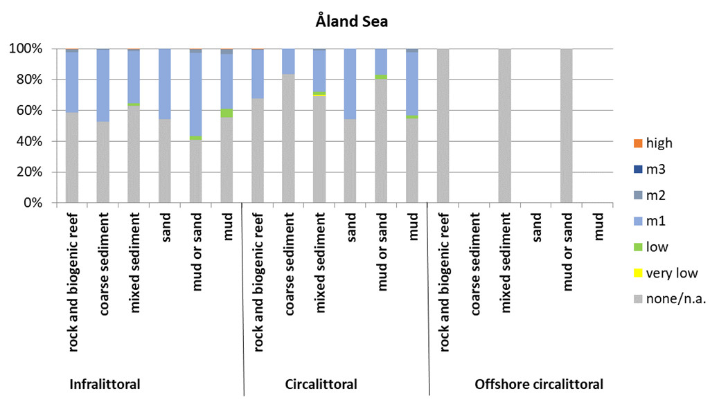
Table 10 Åland Sea
| Infralittoral rock and biogenic reef | Infralittoral coarse sediment | Infralittoral mixed sediment | Infralittoral sand | Infralittoral mud or Infralittoral sand | Infralittoral mud | Circalittoral rock and biogenic reef | Circalittoral coarse sediment | Circalittoral mixed sediment | Circalittoral sand | Circalittoral mud or Circalittoral sand | Circalittoral mud | Offshore circalittoral rock and biogenic reef | Offshore circalittoral coarse sediment | Offshore circalittoral mixed sediment | Offshore circalittoral sand | Offshore circalittoral mud or Offshore circalittoral sand | Offshore circalittoral mud | |
| none | 58.5 | 52.5 | 63.0 | 54.2 | 40.8 | 55.5 | 67.8 | 83.4 | 69.3 | 54.2 | 80.5 | 54.9 | 100 | – | 100 | – | 100 | – |
| very low | 0 | 0 | 0 | 0 | 0 | 0 | 0 | 0 | 0.9 | 0 | 0 | 0 | 0 | – | 0 | – | 0 | – |
| low | <0.1 | 0 | 1.6 | <0.1 | 2.5 | 5.5 | 0 | 0 | 1.7 | 0.3 | 2.7 | 2.0 | 0 | – | 0 | – | 0 | – |
| m1 | 39.4 | 46.8 | 33.7 | 45.3 | 54.0 | 35.4 | 31.3 | 16.6 | 27.2 | 45.6 | 16.4 | 40.9 | 0 | – | 0 | – | 0 | – |
| m2 | 1.9 | 0.7 | 1.5 | 0.3 | 2.3 | 3.1 | 0.8 | <0.1 | 0.9 | 0 | 0.4 | 2.1 | 0 | – | 0 | – | 0 | – |
| m3 | <0.1 | 0 | <0.1 | <0.1 | <0.1 | <0.1 | <0.1 | 0 | <0.1 | 0 | <0.1 | 0 | 0 | – | 0 | – | 0 | – |
| high | 0.2 | <0.1 | 0.2 | <0.1 | 0.4 | 0.5 | 0.2 | 0 | 0.1 | 0 | <0.1 | 0.1 | 0 | – | 0 | – | 0 | – |
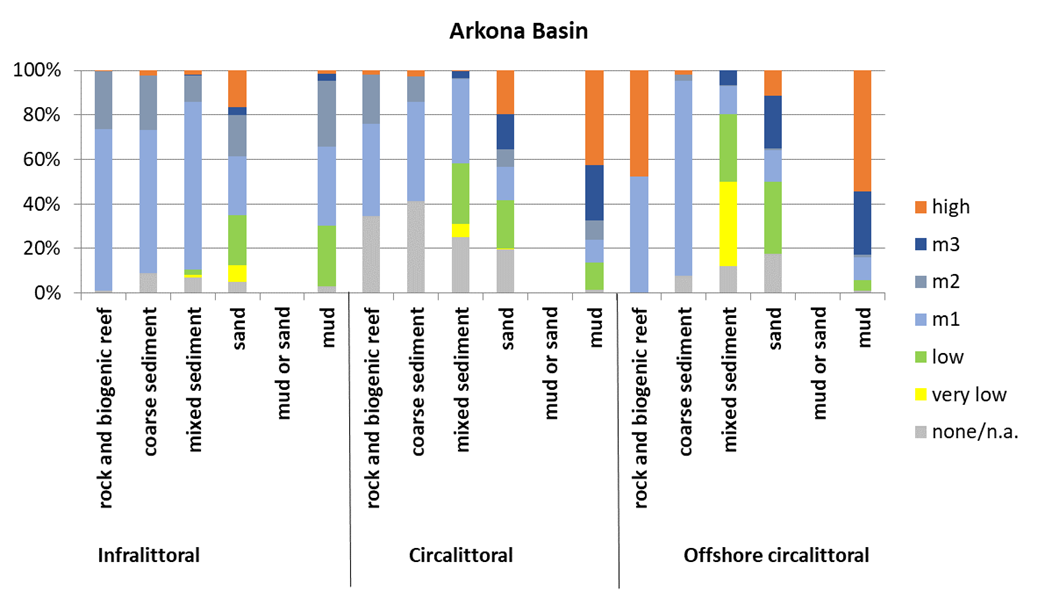
Table 11 Arkona Basin
| Infralittoral rock and biogenic reef | Infralittoral coarse sediment | Infralittoral mixed sediment | Infralittoral sand | Infralittoral mud or Infralittoral sand | Infralittoral mud | Circalittoral rock and biogenic reef | Circalittoral coarse sediment | Circalittoral mixed sediment | Circalittoral sand | Circalittoral mud or Circalittoral sand | Circalittoral mud | Offshore circalittoral rock and biogenic reef | Offshore circalittoral coarse sediment | Offshore circalittoral mixed sediment | Offshore circalittoral sand | Offshore circalittoral mud or Offshore circalittoral sand | Offshore circalittoral mud | |
| none | 0.9 | 8.9 | 6.8 | 4.9 | – | 3.0 | 34.5 | 41.4 | 25.1 | 19.7 | – | 1.5 | 0 | 7.7 | 11.9 | 17.5 | – | 1.0 |
| very low | 0 | 0 | 1.5 | 7.6 | – | 0 | 0 | 0 | 5.8 | 0.3 | – | 0 | 0 | 0 | 38.0 | 0 | – | 0 |
| low | 0 | 0 | 2.2 | 22.6 | – | 27.5 | 0 | 0 | 27.3 | 21.6 | – | 12.1 | 0 | 0 | 30.2 | 32.4 | – | 4.8 |
| m1 | 72.7 | 64.3 | 75.1 | 26.4 | – | 35.4 | 41.4 | 44.4 | 37.9 | 15.0 | – | 10.3 | 52.2 | 87.7 | 12.6 | 14.2 | – | 10.5 |
| m2 | 26.0 | 24.4 | 12.1 | 18.4 | – | 29.3 | 22.2 | 11.6 | 0.4 | 8.1 | – | 8.9 | 0 | 2.5 | 0.4 | 1.0 | – | 1.1 |
| m3 | <0.1 | <0.1 | <0.1 | 3.7 | – | 3.2 | <0.1 | <0.1 | 2.9 | 15.8 | – | 24.7 | 0 | 0 | 6.8 | 23.7 | – | 28.3 |
| high | 0.3 | 2.3 | 2.1 | 16.4 | – | 1.7 | 2.0 | 2.6 | 0.5 | 19.5 | – | 42.6 | 47.8 | 2.1 | <0.1 | 11.3 | – | 54.4 |
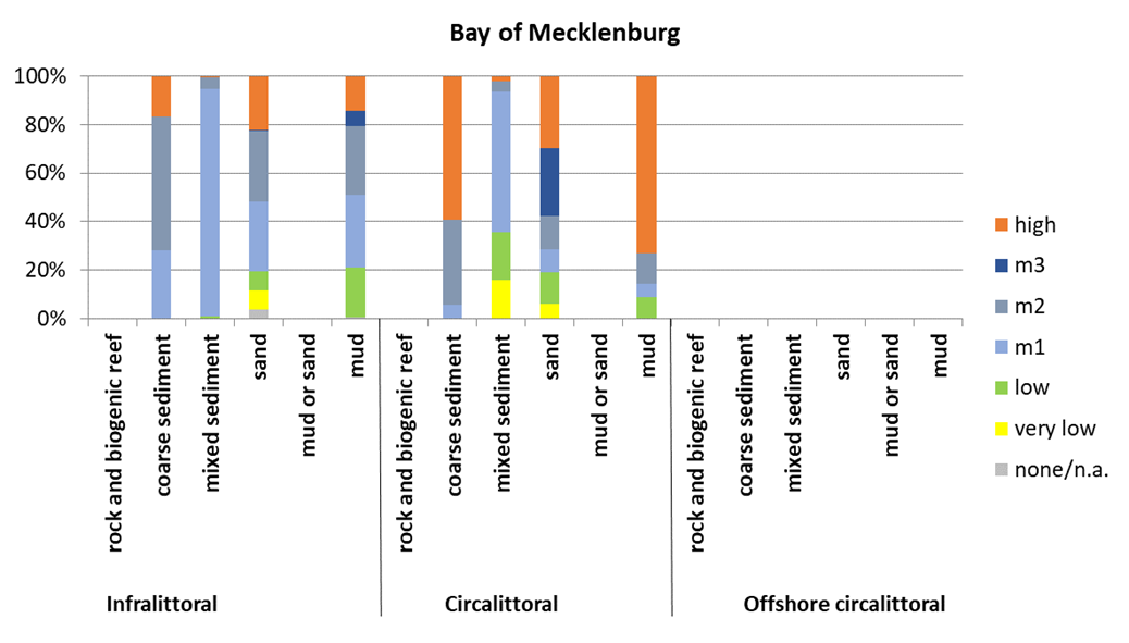
Table 12 Bay of Mecklenburg
| Infralittoral rock and biogenic reef | Infralittoral coarse sediment | Infralittoral mixed sediment | Infralittoral sand | Infralittoral mud or Infralittoral sand | Infralittoral mud | Circalittoral rock and biogenic reef | Circalittoral coarse sediment | Circalittoral mixed sediment | Circalittoral sand | Circalittoral mud or Circalittoral sand | Circalittoral mud | Offshore circalittoral rock and biogenic reef | Offshore circalittoral coarse sediment | Offshore circalittoral mixed sediment | Offshore circalittoral sand | Offshore circalittoral mud or Offshore circalittoral sand | Offshore circalittoral mud | |
| none | – | <0.1 | <0.1 | 3.6 | – | 0.6 | – | 0 | 0 | <0.1 | – | 0 | – | – | – | – | – | – |
| very low | – | 0 | 0 | 8.0 | – | 0 | – | 0 | 15.7 | 6.1 | – | 0 | – | – | – | – | – | – |
| low | – | 0 | 0.7 | 7.7 | – | 20.5 | – | 0 | 20.0 | 13.1 | – | 9.0 | – | – | – | – | – | – |
| m1 | – | 28.3 | 94.0 | 29.0 | – | 29.7 | – | 5.4 | 57.8 | 9.2 | – | 5.2 | – | – | – | – | – | – |
| m2 | – | 54.8 | 4.8 | 29.2 | – | 28.6 | – | 35.4 | 4.2 | 13.8 | – | 12.9 | – | – | – | – | – | – |
| m3 | – | <0.1 | 0 | 0.1 | – | 6.3 | – | 0 | 0 | 27.9 | – | <0.1 | – | – | – | – | – | – |
| high | – | 16.9 | 0.4 | 22.4 | – | 14.2 | – | 59.2 | 2.2 | 29.9 | – | 72.9 | – | – | – | – | – | – |
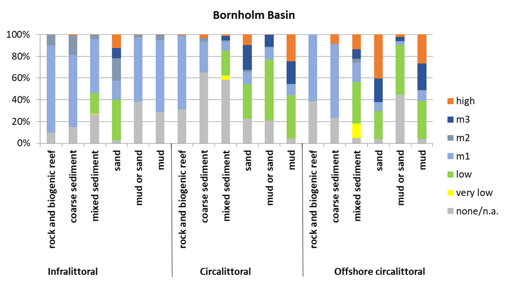
Table 13 Bornholm Basin
| Infralittoral rock and biogenic reef | Infralittoral coarse sediment | Infralittoral mixed sediment | Infralittoral sand | Infralittoral mud or Infralittoral sand | Infralittoral mud | Circalittoral rock and biogenic reef | Circalittoral coarse sediment | Circalittoral mixed sediment | Circalittoral sand | Circalittoral mud or Circalittoral sand | Circalittoral mud | Offshore circalittoral rock and biogenic reef | Offshore circalittoral coarse sediment | Offshore circalittoral mixed sediment | Offshore circalittoral sand | Offshore circalittoral mud or Offshore circalittoral sand | Offshore circalittoral mud | |
| none | 9.8 | 14.9 | 26.9 | 2.6 | 38.2 | 28.8 | 31.1 | 65.3 | 58.2 | 22.4 | 20.8 | 4.4 | 38.5 | 23.4 | 4.9 | 4.1 | 44.5 | 3.9 |
| very low | 0 | 0 | 0.2 | 0.4 | 0 | 0 | 0 | 0 | 4.1 | <0.1 | 0 | 0 | 0 | 0 | 13.1 | 0 | 0 | 0 |
| low | 0 | 0.3 | 18.9 | 37.2 | <0.1 | 0 | 0 | 0 | 22.9 | 31.6 | 56.7 | 39.6 | 0 | 0 | 38.5 | 25.4 | 45.7 | 35.1 |
| m1 | 80.3 | 66.2 | 49.8 | 17.6 | 59.4 | 66.0 | 67.6 | 28.1 | 8.1 | 11.3 | 10.4 | 10.3 | 61.5 | 68.3 | 17.5 | 8.6 | 3.5 | 9.6 |
| m2 | 10.0 | 17.8 | 4.0 | 20.4 | 2.2 | 5.1 | 0.6 | 3.0 | 1.3 | 2.1 | 1.0 | <0.1 | 0 | 0 | 3.5 | 0 | 0 | 0.3 |
| m3 | 0 | <0.1 | 0.1 | 9.2 | 0 | 0 | 0 | 0 | 3.9 | 23.0 | 10.9 | 20.9 | 0 | 0 | 8.9 | 21.6 | 4.0 | 24.6 |
| high | <0.1 | 0.9 | <0.1 | 12.6 | 0.3 | <0.1 | 0.7 | 3.6 | 1.5 | 9.6 | 0.4 | 24.7 | 0 | 8.3 | 13.6 | 40.4 | 2.2 | 26.5 |
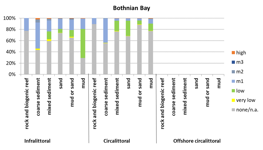
Table 14 Bothnian Bay
| Infralittoral rock and biogenic reef | Infralittoral coarse sediment | Infralittoral mixed sediment | Infralittoral sand | Infralittoral mud or Infralittoral sand | Infralittoral mud | Circalittoral rock and biogenic reef | Circalittoral coarse sediment | Circalittoral mixed sediment | Circalittoral sand | Circalittoral mud or Circalittoral sand | Circalittoral mud | Offshore circalittoral rock and biogenic reef | Offshore circalittoral coarse sediment | Offshore circalittoral mixed sediment | Offshore circalittoral sand | Offshore circalittoral mud or Offshore circalittoral sand | Offshore circalittoral mud | |
| none | 77.6 | 43.6 | 59.4 | 73.4 | 65.2 | 29.1 | 89.2 | 55.4 | 76.4 | 68.1 | 88.2 | 77.0 | – | – | – | – | – | – |
| very low | 0 | 2.1 | 2.9 | 0.7 | 1.6 | <0.1 | 0 | 0.7 | 0.6 | 0.1 | 0.6 | 0.7 | – | – | – | – | – | – |
| low | 0 | 0 | 14.1 | 6.6 | 12.0 | 51.4 | 0 | 0 | 18.3 | 27.1 | 7.1 | 12.7 | – | – | – | – | – | – |
| m1 | 22.4 | 46.5 | 19.5 | 17.9 | 18.0 | 18.6 | 10.8 | 43.2 | 4.0 | 4.3 | 3.3 | 7.7 | – | – | – | – | – | – |
| m2 | 0 | 5.4 | 3.0 | 1.2 | 2.2 | 0.3 | 0 | 0.6 | 0.6 | 0.2 | 0.6 | 1.3 | – | – | – | – | – | – |
| m3 | 0 | 0 | <0.1 | <0.1 | <0.1 | 0 | 0 | 0 | <0.1 | <0.1 | <0.1 | 0 | – | – | – | – | – | – |
| high | 0 | 2.4 | 1.1 | 0.3 | 0.9 | 0.6 | 0 | <0.1 | 0.1 | 0.2 | 0.2 | 0.7 | – | – | – | – | – | – |
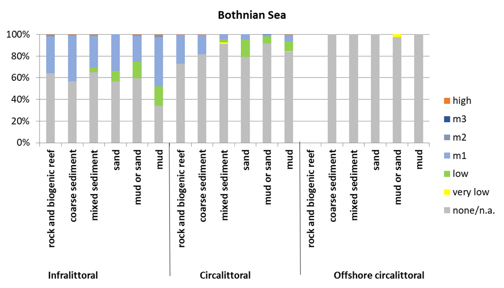
Table 15 Bothnian Sea
| Infralittoral rock and biogenic reef | Infralittoral coarse sediment | Infralittoral mixed sediment | Infralittoral sand | Infralittoral mud or Infralittoral sand | Infralittoral mud | Circalittoral rock and biogenic reef | Circalittoral coarse sediment | Circalittoral mixed sediment | Circalittoral sand | Circalittoral mud or Circalittoral sand | Circalittoral mud | Offshore circalittoral rock and biogenic reef | Offshore circalittoral coarse sediment | Offshore circalittoral mixed sediment | Offshore circalittoral sand | Offshore circalittoral mud or Offshore circalittoral sand | Offshore circalittoral mud | |
| none | 64.4 | 56.6 | 64.9 | 56.8 | 59.6 | 34.5 | 73.0 | 81.5 | 91.0 | 79.1 | 91.7 | 84.2 | – | 100 | 100 | 100 | 97.3 | 100 |
| very low | 0 | 0 | <0.1 | 0 | 0 | 0 | 0 | <0.1 | 1.8 | 0 | 0.1 | <0.1 | – | 0 | <0.1 | 0 | 2.8 | 0 |
| low | 0 | 0 | 4.6 | 9.6 | 15.4 | 17.6 | 0 | 0 | 2.5 | 15.9 | 6.6 | 9.1 | – | 0 | 0 | 0 | 0 | 0 |
| m1 | 33.7 | 42.3 | 29.2 | 33.7 | 23.6 | 45.2 | 26.6 | 18.1 | 4.7 | 5.0 | 1.2 | 6.0 | – | 0 | 0 | 0 | 0 | 0 |
| m2 | 1.6 | 1.0 | 1.1 | 0 | 1.1 | 2.3 | 0.4 | 0.3 | <0.1 | 0 | <0.1 | 0.4 | – | 0 | 0 | 0 | 0 | 0 |
| m3 | 0 | <0.1 | <0.1 | 0 | <0.1 | <0.1 | 0 | 0 | <0.1 | 0 | 0.4 | 0.2 | – | 0 | 0 | 0 | 0 | 0 |
| high | 0.4 | <0.1 | 0.2 | 0 | 0.2 | 0.3 | <0.1 | <0.1 | <0.1 | 0 | <0.1 | <0.1 | – | 0 | 0 | 0 | 0 | 0 |
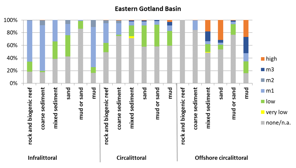
Table 16 Eastern Gotland Basin
| Infralittoral rock and biogenic reef | Infralittoral coarse sediment | Infralittoral mixed sediment | Infralittoral sand | Infralittoral mud or Infralittoral sand | Infralittoral mud | Circalittoral rock and biogenic reef | Circalittoral coarse sediment | Circalittoral mixed sediment | Circalittoral sand | Circalittoral mud or Circalittoral sand | Circalittoral mud | Offshore circalittoral rock and biogenic reef | Offshore circalittoral coarse sediment | Offshore circalittoral mixed sediment | Offshore circalittoral sand | Offshore circalittoral mud or Offshore circalittoral sand | Offshore circalittoral mud | |
| none | 18.4 | 17.8 | 38.5 | 42.6 | 86.3 | 16.7 | 49.2 | 74.9 | 71.2 | 57.8 | 58.3 | 59.6 | 100 | 84.4 | 48.4 | 53.5 | 76.7 | 15.9 |
| very low | 0 | 0 | 0 | 0 | 0 | 0 | 0 | 0 | 3.4 | 0 | 0 | 0 | 0 | 0 | 1.1 | 0 | 0 | 0 |
| low | 15.8 | 1.8 | 27.5 | 33.3 | 12.1 | 8.9 | 14.5 | 2.0 | 16.6 | 33.5 | 34.2 | 23.1 | 0 | 0 | 12.4 | 7.6 | 16.8 | 18.7 |
| m1 | 64.8 | 72.3 | 33.9 | 18.1 | 1.4 | 63.4 | 31.3 | 18.0 | 6.6 | 5.9 | 5.7 | 8.5 | 0 | 15.1 | 4.5 | 2.9 | 3.9 | 13.1 |
| m2 | 1.0 | 7.9 | <0.1 | 6.0 | <0.1 | 11.1 | 4.6 | 4.5 | <0.1 | 0.6 | 0.4 | 0 | 0 | 0 | <0.1 | 0 | 0 | 0 |
| m3 | 0 | <0.1 | 0 | <0.1 | <0.1 | 0 | 0 | 0 | 1.3 | 1.4 | 1.3 | 5.5 | 0 | 0 | 15.2 | 4.6 | 2.1 | 25.7 |
| high | <0.1 | 0.2 | <0.1 | <0.1 | <0.1 | 0 | 0.4 | 0.6 | 0.8 | 0.8 | <0.1 | 3.2 | 0 | 0.4 | 18.2 | 31.4 | 0.6 | 26.6 |
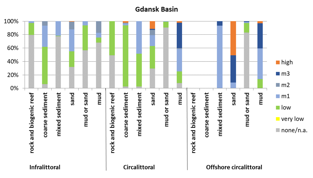
Table 17 Gdansk Basin
| Infralittoral rock and biogenic reef | Infralittoral coarse sediment | Infralittoral mixed sediment | Infralittoral sand | Infralittoral mud or Infralittoral sand | Infralittoral mud | Circalittoral rock and biogenic reef | Circalittoral coarse sediment | Circalittoral mixed sediment | Circalittoral sand | Circalittoral mud or Circalittoral sand | Circalittoral mud | Offshore circalittoral rock and biogenic reef | Offshore circalittoral coarse sediment | Offshore circalittoral mixed sediment | Offshore circalittoral sand | Offshore circalittoral mud or Offshore circalittoral sand | Offshore circalittoral mud | |
| none | 79.5 | 6.3 | 77.6 | 31.7 | 56.8 | 68.1 | 49.1 | 2.6 | 2.6 | 29.5 | 90.8 | 7.9 | – | – | 0 | 0 | 83.1 | 0 |
| very low | 0 | 0 | 0 | 0 | 0 | 0 | 0 | 0 | 0 | 0 | 0 | 0 | – | – | 0 | 0 | 0 | 0 |
| low | 18.0 | 55.6 | 0.9 | 23.6 | 36.9 | 7.6 | 50.9 | 91.4 | 49.0 | 33.7 | 8.6 | 17.3 | – | – | 0 | 0 | 14.2 | 13.7 |
| m1 | 2.5 | 31.4 | 21.5 | 32.8 | 6.4 | 7.1 | 0 | 2.6 | 48.4 | 16.2 | 0.5 | 33.7 | – | – | 93.4 | 8.6 | 1.6 | 45.8 |
| m2 | 0 | 6.8 | 0 | 11.2 | 0 | 17.2 | 0 | 1.2 | 0 | 7.8 | 0 | 0.9 | – | – | 0 | 0 | 0 | 0 |
| m3 | 0 | 0 | 0 | <0.1 | 0 | 0 | 0 | 0 | 0 | 1.3 | 0 | 38.1 | – | – | 6.6 | 40.7 | 1.2 | 37.6 |
| high | 0 | 0 | 0 | 0.7 | 0 | 0 | 0 | 2.3 | 0 | 11.5 | 0 | 2.1 | – | – | 0 | 50.7 | 0 | 2.9 |
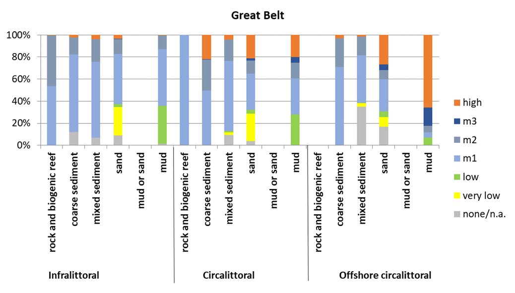
Table 18 Great Belt
| Infralittoral rock and biogenic reef | Infralittoral coarse sediment | Infralittoral mixed sediment | Infralittoral sand | Infralittoral mud or Infralittoral sand | Infralittoral mud | Circalittoral rock and biogenic reef | Circalittoral coarse sediment | Circalittoral mixed sediment | Circalittoral sand | Circalittoral mud or Circalittoral sand | Circalittoral mud | Offshore circalittoral rock and biogenic reef | Offshore circalittoral coarse sediment | Offshore circalittoral mixed sediment | Offshore circalittoral sand | Offshore circalittoral mud or Offshore circalittoral sand | Offshore circalittoral mud | |
| none | 0.2 | 12.1 | 6.8 | 8.9 | – | 1.6 | 0 | 0.3 | 9.3 | 3.7 | – | 0.4 | – | 0 | 35.2 | 17.0 | – | 0 |
| very low | 0 | 0 | <0.1 | 25.8 | – | 0 | 0 | 0 | 2.6 | 24.8 | – | 0 | – | 0 | 3.1 | 8.6 | – | 0 |
| low | 0 | 0 | <0.1 | 2.7 | – | 34.2 | 0 | 0 | 1.0 | 3.8 | – | 27.6 | – | 0 | 0.4 | 5.2 | – | 7.0 |
| m1 | 53.2 | 70.2 | 68.6 | 45.4 | – | 51.5 | 100 | 49.2 | 63.3 | 32.6 | – | 32.8 | – | 71.0 | 43.0 | 29.3 | – | 4.6 |
| m2 | 46.4 | 15.2 | 20.5 | 13.2 | – | 12.6 | 0 | 28.0 | 19.5 | 11.8 | – | 14.3 | – | 25.8 | 16.6 | 8.3 | – | 5.9 |
| m3 | 0 | <0.1 | <0.1 | 0.4 | – | <0.1 | 0 | 0.3 | 0 | 2.1 | – | 4.8 | – | 0 | 0 | 5.1 | – | 16.7 |
| high | 0.3 | 2.4 | 4.0 | 3.6 | – | 0.2 | 0 | 22.1 | 4.3 | 21.2 | – | 20.2 | – | 3.3 | 1.7 | 26.6 | – | 65.8 |
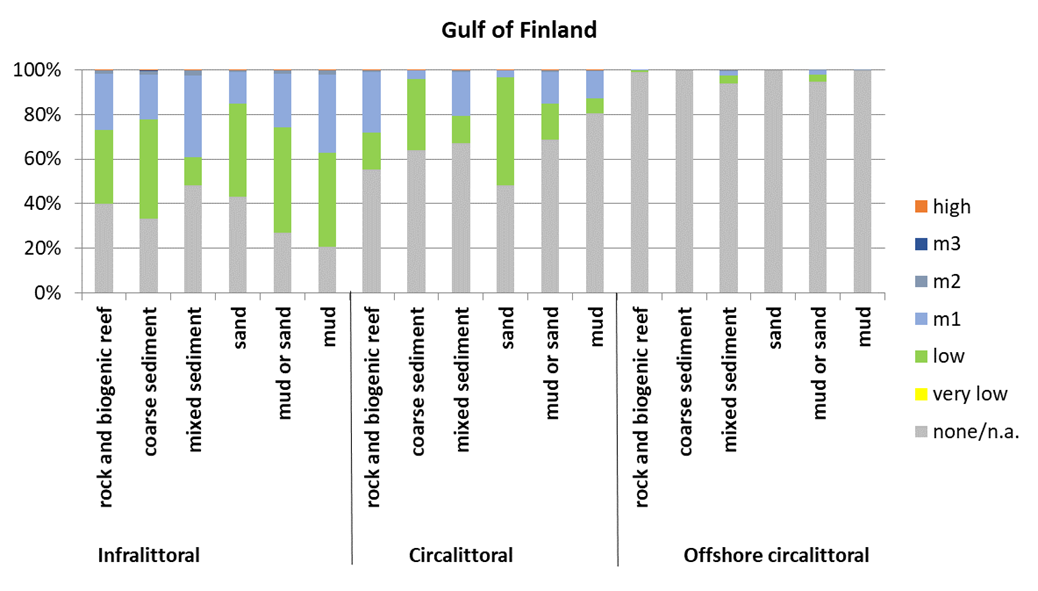
Table 19 Gulf of Finland
| Infralittoral rock and biogenic reef | Infralittoral coarse sediment | Infralittoral mixed sediment | Infralittoral sand | Infralittoral mud or Infralittoral sand | Infralittoral mud | Circalittoral rock and biogenic reef | Circalittoral coarse sediment | Circalittoral mixed sediment | Circalittoral sand | Circalittoral mud or Circalittoral sand | Circalittoral mud | Offshore circalittoral rock and biogenic reef | Offshore circalittoral coarse sediment | Offshore circalittoral mixed sediment | Offshore circalittoral sand | Offshore circalittoral mud or Offshore circalittoral sand | Offshore circalittoral mud | |
| none | 40.1 | 33.2 | 48.3 | 43.0 | 26.9 | 20.7 | 55.3 | 63.8 | 67.2 | 48.1 | 68.8 | 80.5 | 98.9 | 100 | 93.8 | 100 | 94.8 | 99.7 |
| very low | 0 | 0 | 0 | 0 | 0 | 0 | 0 | 0 | 0 | 0 | 0 | 0 | 0 | 0 | 0 | 0 | 0 | 0 |
| low | 32.9 | 44.7 | 12.5 | 42.0 | 47.5 | 42.1 | 16.6 | 32.2 | 12.3 | 48.7 | 16.1 | 6.6 | 1.0 | 0 | 3.7 | 0 | 2.9 | 0.2 |
| m1 | 25.5 | 19.9 | 36.7 | 14.2 | 23.8 | 35.2 | 27.1 | 3.7 | 19.4 | 2.9 | 14.4 | 12.4 | 0.1 | 0 | 2.2 | 0 | 2.0 | <0.1 |
| m2 | 1.4 | 1.8 | 2.2 | 0.5 | 1.4 | 1.9 | 1.0 | 0.1 | 1.0 | <0.1 | 0.7 | 0.5 | 0 | 0 | 0.4 | 0 | 0.3 | <0.1 |
| m3 | <0.1 | 0.1 | <0.1 | <0.1 | 0.1 | <0.1 | <0.1 | <0.1 | <0.1 | <0.1 | <0.1 | <0.1 | 0 | 0 | 0 | 0 | 0 | 0 |
| high | 0.2 | 0.3 | 0.2 | 0.2 | 0.2 | <0.1 | <0.1 | <0.1 | <0.1 | <0.1 | <0.1 | <0.1 | 0 | 0 | 0 | 0 | 0 | 0 |
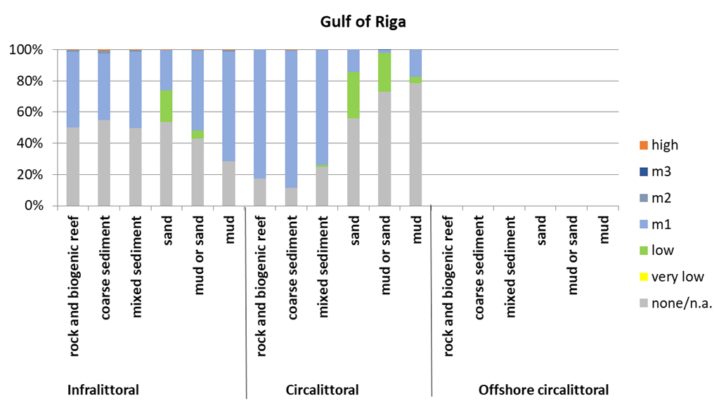
Table 20 Gulf of Riga
| Infralittoral rock and biogenic reef | Infralittoral coarse sediment | Infralittoral mixed sediment | Infralittoral sand | Infralittoral mud or Infralittoral sand | Infralittoral mud | Circalittoral rock and biogenic reef | Circalittoral coarse sediment | Circalittoral mixed sediment | Circalittoral sand | Circalittoral mud or Circalittoral sand | Circalittoral mud | Offshore circalittoral rock and biogenic reef | Offshore circalittoral coarse sediment | Offshore circalittoral mixed sediment | Offshore circalittoral sand | Offshore circalittoral mud or Offshore circalittoral sand | Offshore circalittoral mud | |
| none | 50.0 | 54.7 | 49.8 | 53.7 | 43.0 | 28.5 | 17.4 | 11.4 | 24.9 | 56.1 | 72.9 | 78.4 | – | – | – | – | – | – |
| very low | 0 | 0 | 0 | 0 | 0 | 0 | 0 | 0 | 0 | 0 | 0 | 0 | – | – | – | – | – | – |
| low | 0 | 0 | <0.1 | 20.1 | 5.2 | <0.1 | 0 | 0 | 1.2 | 29.4 | 24.8 | 3.9 | – | – | – | – | – | – |
| m1 | 48.5 | 42.5 | 48.9 | 25.9 | 51.2 | 70.3 | 82.6 | 87.9 | 73.7 | 14.6 | 2.2 | 17.7 | – | – | – | – | – | – |
| m2 | 1.4 | 2.3 | 1.0 | 0.3 | 0.5 | 1.1 | 0 | 0.7 | 0.1 | 0 | 0 | <0.1 | – | – | – | – | – | – |
| m3 | 0 | <0.1 | <0.1 | <0.1 | 0 | 0 | 0 | 0 | <0.1 | <0.1 | <0.1 | 0 | – | – | – | – | – | – |
| high | 0.1 | 0.5 | 0.3 | <0.1 | 0.1 | 0.2 | 0 | 0.1 | <0.1 | <0.1 | <0.1 | <0.1 | – | – | – | – | – | – |
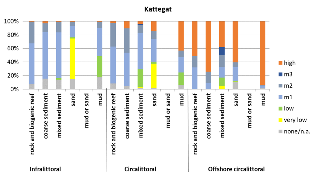
Table 21 Kattegat
| Infralittoral rock and biogenic reef | Infralittoral coarse sediment | Infralittoral mixed sediment | Infralittoral sand | Infralittoral mud or Infralittoral sand | Infralittoral mud | Circalittoral rock and biogenic reef | Circalittoral coarse sediment | Circalittoral mixed sediment | Circalittoral sand | Circalittoral mud or Circalittoral sand | Circalittoral mud | Offshore circalittoral rock and biogenic reef | Offshore circalittoral coarse sediment | Offshore circalittoral mixed sediment | Offshore circalittoral sand | Offshore circalittoral mud or Offshore circalittoral sand | Offshore circalittoral mud | |
| none | 7.2 | 15.4 | 14.0 | 15.2 | – | 17.3 | 8.4 | 5.0 | 2.2 | 1.9 | – | 6.4 | 0.4 | <0.1 | 0.7 | 10.8 | – | 1.9 |
| very low | 0 | 0 | 0 | 59.3 | – | 0 | 0 | 0 | 1.0 | 35.5 | – | 0 | 0 | 0 | 4.1 | 0.5 | – | 0 |
| low | 0 | <0.1 | 2.2 | 2.0 | – | 31.2 | 0 | <0.1 | 26.2 | 3.0 | – | 18.0 | 0 | 0 | 12.1 | <0.1 | – | <0.1 |
| m1 | 60.3 | 68.6 | 67.6 | 16.9 | – | 41.3 | 54.5 | 48.9 | 53.5 | 33.7 | – | 22.9 | 31.5 | 9.1 | 15.9 | 21.1 | – | 3.1 |
| m2 | 32.1 | 13.0 | 15.2 | 5.8 | – | 9.0 | 34.4 | 35.5 | 11.6 | 11.1 | – | 9.4 | 16.5 | 16.6 | 17.9 | 7.1 | – | 1.2 |
| m3 | 0 | <0.1 | <0.1 | <0.1 | – | 0.3 | 0 | <0.1 | 1.8 | <0.1 | – | <0.1 | 0 | 0 | 11.5 | 0 | – | <0.1 |
| high | 0.4 | 3.0 | 0.9 | 0.9 | – | 0.9 | 2.7 | 10.6 | 3.7 | 14.9 | – | 43.3 | 51.6 | 74.2 | 37.9 | 60.4 | – | 93.8 |
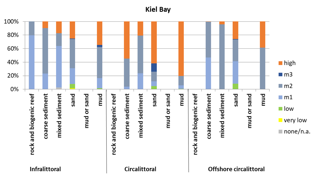
Table 22 Kiel Bay
| Infralittoral rock and biogenic reef | Infralittoral coarse sediment | Infralittoral mixed sediment | Infralittoral sand | Infralittoral mud or Infralittoral sand | Infralittoral mud | Circalittoral rock and biogenic reef | Circalittoral coarse sediment | Circalittoral mixed sediment | Circalittoral sand | Circalittoral mud or Circalittoral sand | Circalittoral mud | Offshore circalittoral rock and biogenic reef | Offshore circalittoral coarse sediment | Offshore circalittoral mixed sediment | Offshore circalittoral sand | Offshore circalittoral mud or Offshore circalittoral sand | Offshore circalittoral mud | |
| none | 0 | <0.1 | 2.8 | <0.1 | – | <0.1 | – | 0 | 0 | <0.1 | – | 0 | – | 0 | 0 | 0 | – | 0 |
| very low | 0 | 0 | <0.1 | 1.4 | – | 0 | – | 0 | 0 | <0.1 | – | 0 | – | 0 | 0 | 0 | – | 0 |
| low | 0 | 0 | 0 | 6.4 | – | 1.4 | – | 0 | 0 | 4.4 | – | 0.8 | – | 0 | 0 | 8.4 | – | 0 |
| m1 | 79.6 | 23.3 | 61.1 | 23.3 | – | 14.9 | – | 4.0 | 23.6 | 7.4 | – | 4.9 | – | 46.8 | 0 | 33.2 | – | 0 |
| m2 | 20.4 | 66.9 | 18.6 | 42.8 | – | 46.1 | – | 41.4 | 55.5 | 14.2 | – | 13.9 | – | 52.9 | 95.8 | 31.9 | – | 61.3 |
| m3 | 0 | <0.1 | 0 | 1.0 | – | 3.1 | – | 0 | 0 | 12.1 | – | <0.1 | – | 0 | 0 | 0.7 | – | 0 |
| high | 0 | 9.8 | 17.5 | 25.0 | – | 34.5 | – | 54.6 | 20.9 | 61.9 | – | 80.3 | – | 0.3 | 4.3 | 25.9 | – | 38.7 |
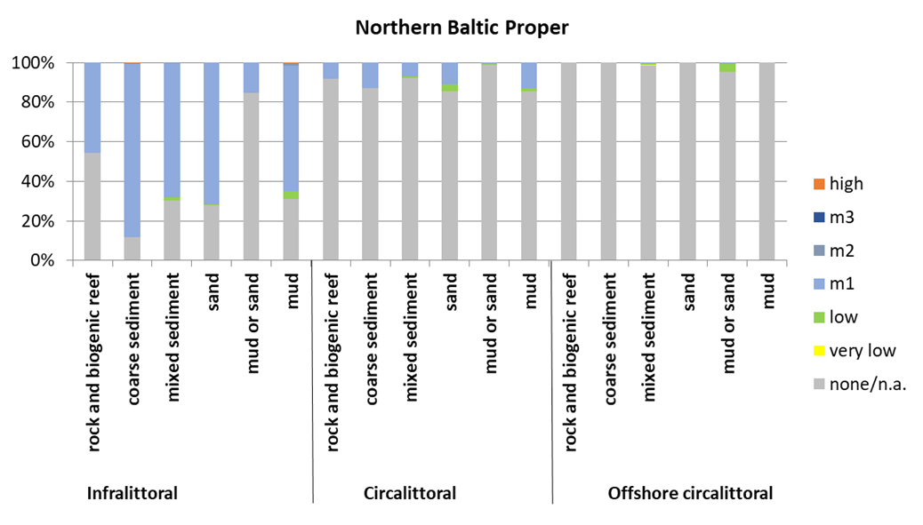
Table 23 Norther Baltic Proper
| Infralittoral rock and biogenic reef | Infralittoral coarse sediment | Infralittoral mixed sediment | Infralittoral sand | Infralittoral mud or Infralittoral sand | Infralittoral mud | Circalittoral rock and biogenic reef | Circalittoral coarse sediment | Circalittoral mixed sediment | Circalittoral sand | Circalittoral mud or Circalittoral sand | Circalittoral mud | Offshore circalittoral rock and biogenic reef | Offshore circalittoral coarse sediment | Offshore circalittoral mixed sediment | Offshore circalittoral sand | Offshore circalittoral mud or Offshore circalittoral sand | Offshore circalittoral mud | |
| none | 54.3 | 11.9 | 30.4 | 27.8 | 84.7 | 31.0 | 92.0 | 87.1 | 92.1 | 85.7 | 98.7 | 85.4 | 100 | 100 | 98.6 | 100 | 95.2 | 100 |
| very low | 0 | 0 | 0 | 0 | 0 | 0 | 0 | 0 | <0.1 | 0 | 0 | 0 | 0 | 0 | 0.4 | 0 | 0 | 0 |
| low | 0 | 0 | 1.3 | 0.7 | 0 | 3.9 | 0 | 0 | 0.8 | 3.2 | 0.4 | 1.6 | 0 | 0 | 0.6 | 0 | 3.9 | 0 |
| m1 | 45.7 | 87.3 | 68.0 | 71.5 | 15.4 | 63.5 | 8.0 | 12.9 | 7.1 | 11.1 | 0.8 | 13.0 | 0 | 0 | 0.3 | 0 | 0.8 | 0 |
| m2 | <0.1 | 0.7 | 0.3 | 0 | 0 | 1.4 | 0 | <0.1 | <0.1 | 0 | 0 | <0.1 | 0 | 0 | <0.1 | 0 | <0.1 | 0 |
| m3 | 0 | <0.1 | <0.1 | 0 | 0 | <0.1 | 0 | 0 | 0 | 0 | 0 | <0.1 | 0 | 0 | 0 | 0 | 0 | 0 |
| high | 0 | 0.1 | <0.1 | 0 | 0 | 0.1 | 0 | <0.1 | 0 | 0 | 0 | <0.1 | 0 | 0 | 0 | 0 | 0 | 0 |
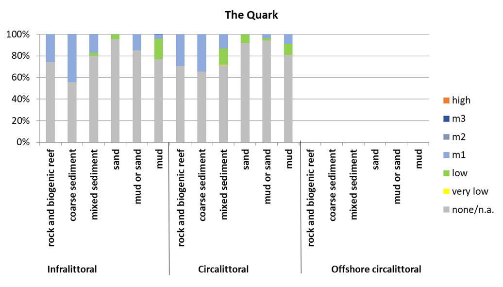
Table 24 The Quark
| Infralittoral rock and biogenic reef | Infralittoral coarse sediment | Infralittoral mixed sediment | Infralittoral sand | Infralittoral mud or Infralittoral sand | Infralittoral mud | Circalittoral rock and biogenic reef | Circalittoral coarse sediment | Circalittoral mixed sediment | Circalittoral sand | Circalittoral mud or Circalittoral sand | Circalittoral mud | Offshore circalittoral rock and biogenic reef | Offshore circalittoral coarse sediment | Offshore circalittoral mixed sediment | Offshore circalittoral sand | Offshore circalittoral mud or Offshore circalittoral sand | Offshore circalittoral mud | |
| none | 74.1 | 55.5 | 80.1 | 95.5 | 85.2 | 76.8 | 70.5 | 65.5 | 71.4 | 91.9 | 94.4 | 80.7 | – | – | – | – | – | – |
| very low | 0 | 0 | 0 | 0 | 0 | 0 | 0 | 0 | 0.5 | 0 | 0 | 0 | – | – | – | – | – | – |
| low | 0 | 0 | 2.8 | 4.4 | 0 | 18.8 | 0 | 0 | 14.8 | 7.8 | 1.8 | 10.2 | – | – | – | – | – | – |
| m1 | 25.9 | 44.2 | 17.0 | 0.1 | 14.8 | 4.3 | 29.5 | 34.6 | 13.4 | 0.3 | 3.9 | 9.1 | – | – | – | – | – | – |
| m2 | 0 | 0.3 | 0.1 | 0 | 0 | 0 | 0 | <0.1 | <0.1 | 0 | 0 | 0 | – | – | – | – | – | – |
| m3 | 0 | 0 | 0 | 0 | 0 | <0.1 | 0 | 0 | 0 | 0 | 0 | 0 | – | – | – | – | – | – |
| high | 0 | <0.1 | 0 | 0 | 0 | <0.1 | 0 | <0.1 | 0 | 0 | 0 | 0 | – | – | – | – | – | – |
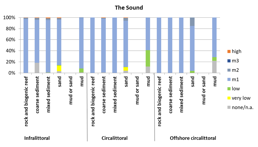
Table 25 The Sound
| Infralittoral rock and biogenic reef | Infralittoral coarse sediment | Infralittoral mixed sediment | Infralittoral sand | Infralittoral mud or Infralittoral sand | Infralittoral mud | Circalittoral rock and biogenic reef | Circalittoral coarse sediment | Circalittoral mixed sediment | Circalittoral sand | Circalittoral mud or Circalittoral sand | Circalittoral mud | Offshore circalittoral rock and biogenic reef | Offshore circalittoral coarse sediment | Offshore circalittoral mixed sediment | Offshore circalittoral sand | Offshore circalittoral mud or Offshore circalittoral sand | Offshore circalittoral mud | |
| none | 0 | 18.3 | 0.4 | 3.2 | – | 0.7 | 0 | 0.7 | 0.2 | 4.1 | – | 11.4 | 0 | <0.1 | 0 | 0 | – | 21.6 |
| very low | 0 | 0 | 0 | 9.9 | – | 0 | 0 | 0 | 0 | 6.2 | – | 0 | 0 | 0 | 0 | 0 | – | 0 |
| low | 0 | 0 | 0.2 | 1.1 | – | 7.3 | 0 | 0 | 0 | 0.5 | – | 29.8 | 0 | 0 | 0 | 3.7 | – | 6.8 |
| m1 | 97.3 | 77.6 | 94.9 | 81.9 | – | 91.6 | 100 | 97.4 | 99.8 | 83.7 | – | 58.5 | 100 | 100 | 100 | 81.1 | – | 71.6 |
| m2 | 2.5 | 3.6 | 3.1 | 3.1 | – | 0.4 | 0 | 1.2 | 0 | 5.0 | – | 0.4 | 0 | 0 | 0 | 15.2 | – | 0 |
| m3 | 0 | <0.1 | <0.1 | <0.1 | – | <0.1 | 0 | 0 | 0 | 0 | – | 0 | 0 | 0 | 0 | 0 | – | 0 |
| high | 0.3 | 0.5 | 1.3 | 0.8 | – | <0.1 | 0 | 0.7 | 0 | 0.6 | – | 0 | 0 | 0 | 0 | 0 | – | 0 |
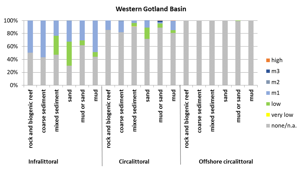
Table 26 Western Gotland Basin
| Infralittoral rock and biogenic reef | Infralittoral coarse sediment | Infralittoral mixed sediment | Infralittoral sand | Infralittoral mud or Infralittoral sand | Infralittoral mud | Circalittoral rock and biogenic reef | Circalittoral coarse sediment | Circalittoral mixed sediment | Circalittoral sand | Circalittoral mud or Circalittoral sand | Circalittoral mud | Offshore circalittoral rock and biogenic reef | Offshore circalittoral coarse sediment | Offshore circalittoral mixed sediment | Offshore circalittoral sand | Offshore circalittoral mud or Offshore circalittoral sand | Offshore circalittoral mud | |
| none | 50.5 | 43.2 | 47.4 | 30.3 | 62.0 | 43.9 | 85.6 | 82.0 | 90.8 | 71.6 | 88.8 | 80.9 | 100 | 100 | 100 | 100 | 99.4 | 100 |
| very low | 0 | 0 | 0 | 0 | 0 | 0 | 0 | 0 | 0.6 | 0 | 0 | 0 | 0 | 0 | 0 | 0 | 0 | 0 |
| low | 0 | 0 | 29.1 | 37.1 | 7.4 | 7.4 | 0 | 0 | 4.7 | 17.5 | 6.6 | 4.3 | 0 | 0 | 0 | 0 | 0.6 | <0.1 |
| m1 | 49.3 | 56.3 | 23.3 | 32.0 | 30.6 | 48.4 | 14.4 | 17.0 | 3.7 | 10.7 | 1.7 | 14.4 | 0 | 0 | 0 | 0 | 0 | 0 |
| m2 | 0.2 | 0.5 | 0.2 | 0.5 | <0.1 | 0.3 | <0.1 | 0.9 | 0.1 | 0 | 0.3 | <0.1 | 0 | 0 | 0 | 0 | 0 | 0 |
| m3 | 0 | <0.1 | <0.1 | <0.1 | <0.1 | 0 | 0 | 0 | <0.1 | 0.2 | 2.1 | 0.2 | 0 | 0 | 0 | 0 | 0 | 0 |
| high | <0.1 | <0.1 | <0.1 | <0.1 | <0.1 | <0.1 | <0.1 | 0.1 | <0.1 | 0 | 0.5 | 0.2 | 0 | 0 | 0 | 0 | 0 | 0 |
A test case was carried out for the German Baltic Sea region in March 2023 based on the HELCOM HOLAS III pressure data, applying settings described in the main text of the indicator report. To test the evaluation procedure of the indicator, the case study for the CumI evaluation was carried out based on two different biotope maps: the EUSeaMap as described in section 9.2 “Methodology applied” (also used for the HOLAS III evaluation) and the current German BHT map which is based on more detailed data mostly from direct biotope mapping surveys. To show the effect of the different distribution of the BHTs and their subsequent sensitivity distribution, the step of applying layers of benthic species leading to high sensitivities was omitted. This prevents masking the differences coming from the BHT maps as the overlay with the species distributions would result in high sensitivities in both maps and thus hide the differences in the respective maps.
Biotopes[4] of the German Baltic Sea (see below) are shown as benthic Broad Habitats based on the EUSeaMap and the current German BHT map (March 2023). While the EUSeaMap does not cover the complete German marine area, the German BHT map also includes coastal water bodies according to WFD/HELCOM Assessment Unit Level 4 such as the inner fjord of Kiel. In contrast to the EUSeaMap, differentiating between the circalittoral and offshore zone, the German BHT map only uses the circalittoral zone.
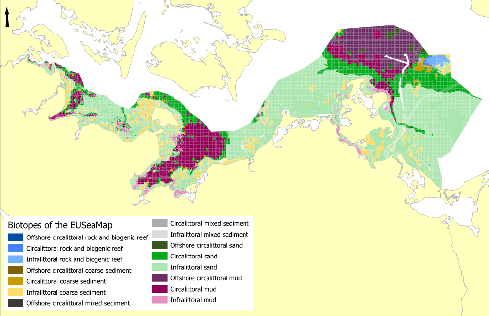
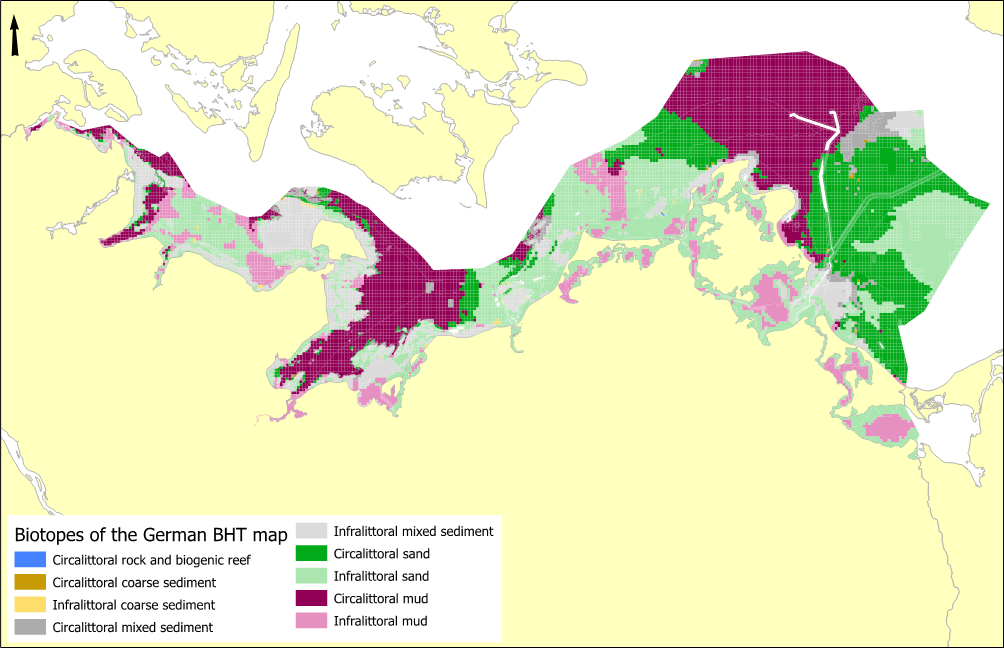
Biotope maps of the German Baltic Sea, showing MSFD benthic Broad Habitat according to the HELCOM EUSeaMap (top) and the national German BHT map (below).
While EUSeaMap is modelled based on available data regarding the underlying sediment and geological information, the German BHT map is based on analyses of national information of abiotic and biotic data as well as mapped areas such as habitat types (in terms of the natural habitat types of the Habitats Directive), which are ultimately mapped the specific MSFD benthic Broad Habitat Types: “rock and biogenic reef”, “coarse sediment”, “mixed sediment”, “sand” and “mud”. The figure below shows the difference in the resulting spatial extent of the habitat types.
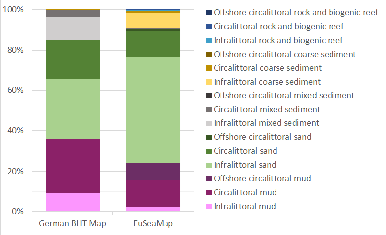
Spatial biotope extent (%) showing MSFD broad scale habitat types in the German Baltic Sea, according to the national German BHT map and the HELCOM EUSeaMap
Based on the biotope maps, the pressure-specific sensitivities were used according to the procedure described in the methodology of the main report.
Sensitivities for surface abrasion (for bottom trawling fishery) and general biotope sensitivity for physical pressures (except fishery) were allocated to each BHT in the infra – and circalittoral zone considering oligo-, meso- or polyhaline salinity conditions (see Appendix G). If an assignment to either a biotope and/or a salinity range was missing, both sensitivities were set to “moderate” (not listed in Appendix G). The resulting sensitivity towards bottom trawling is shown in the map below.
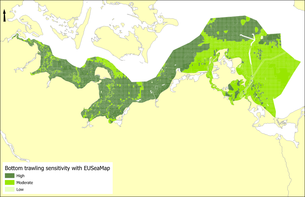
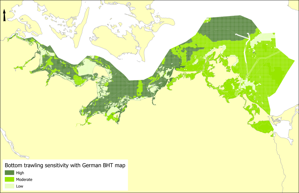
Biotope sensitivities for surface abrasion caused by bottom trawling fishery for benthic Broad Habitat Types according to EUSeaMap (top) and German BHT map (below) in the German Baltic Sea region.
The overall patterns of biotope sensitivities to surface abrasion are similar in both maps. However, in coastal regions and the north-eastern part of the Arkona Basin the German BHT map demonstrates lower bottom trawling sensitivities. Most of the difference can be explained by the underlying biotope/BHT assignment: near the coast to “infralittoral mixed sediments” (German BHT map) opposed to “infralittoral coarse sediments” (EUSeaMap) and in the Arkona basin to “mixed sediment” (German BHT map) versus “coarse sediment“ and “rock and biogenic reef” (EUSeaMap).
Bottom trawling fishery impact
The pressure layers such as fishery data used for this case study are the same as the ones for the Baltic-wide HELCOM assessment. Both EUSeaMap and German BHT map carrying biotope sensitivities are (among other pressures) evaluated against surface abrasion pressure by fishery in the German Baltic Sea. The resulting maps showing only potential fishery impact reveal a similar pattern where most parts of the Arkona basin and the Mecklenburger Bay as well as big areas of the Kieler Bay are potentially impacted by physical disturbance caused by bottom trawling fishery, irrespective of which biotope map was used for the evaluation. Differences in the distribution of the fishery impact are seen mainly in coastal areas and the north-eastern part of the Arkona Basin, where lower fishery/surface abrasion impact in the German BHT map can be explained by the lower sensitivity of the assigned biotopes (compare German BHT maps: trawling impact and trawling sensitivity).
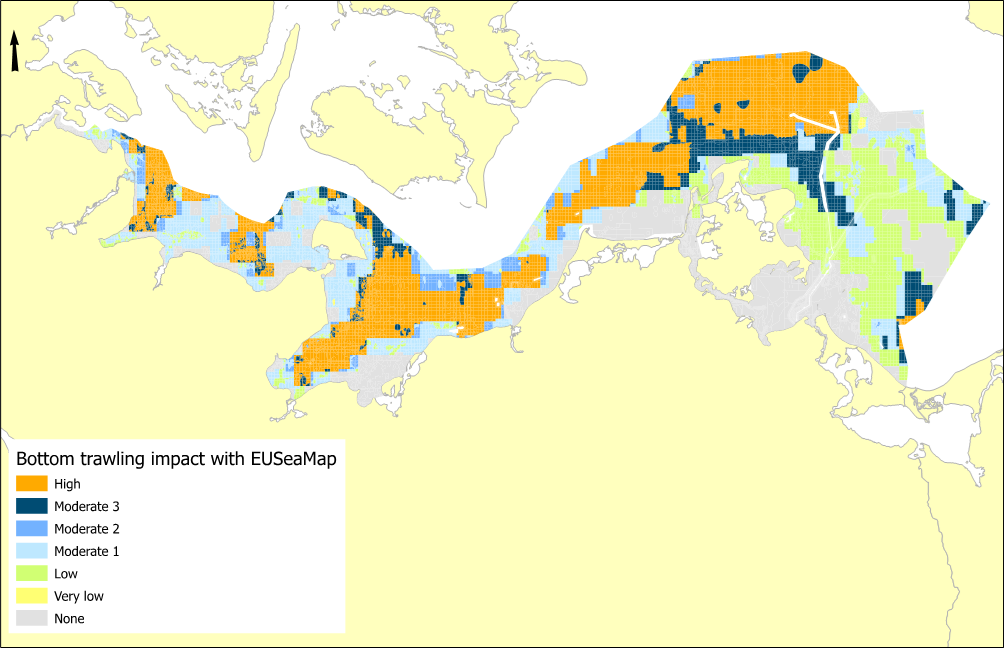
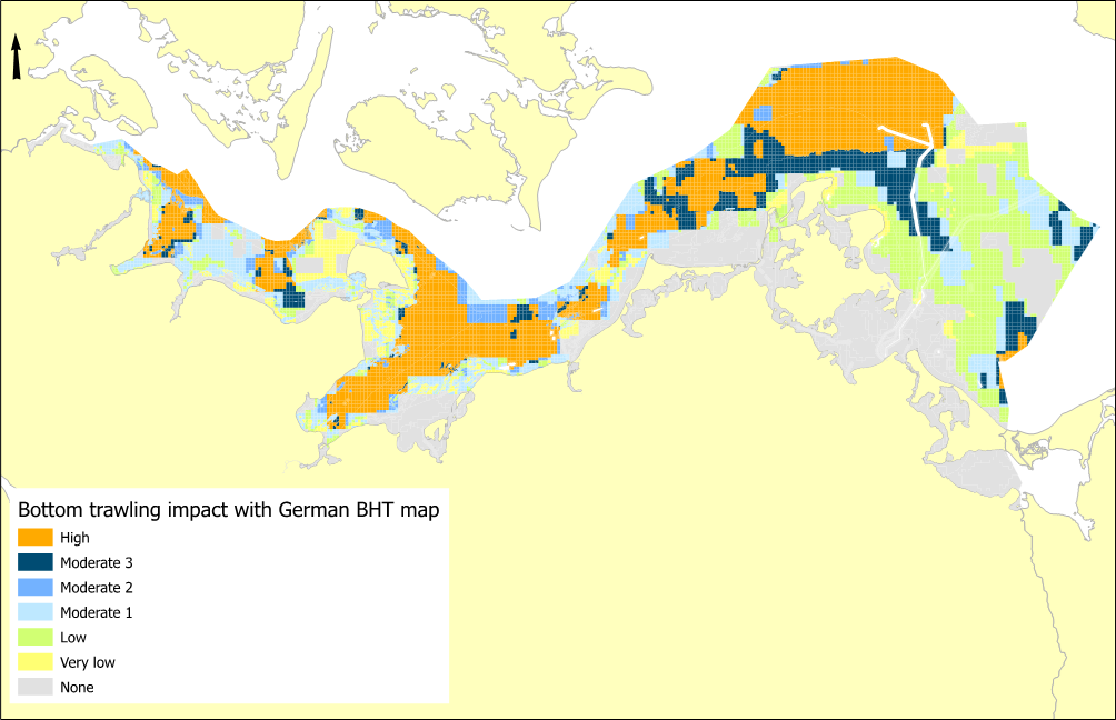
Impact evaluation results of surface abrasion caused by bottom trawling fishery on benthic biotopes indicator in the German Baltic Sea, using benthic Broad Habitat Types according to EUSeaMap (top) and German BHT map (below).
The resulting maps for the cumulative physical disturbance (using all pressure layers) show that more than 25 % of the total German Baltic Sea area is potentially affected to a high degree (see below) and patterns are similar, irrespective of BHT map used (German BHT map or EUSeaMap). Both evaluation maps predict high impact levels in most of the Bay of Mecklenburg, the Arkona Basin (except for the north-eastern area) and major parts of the Kiel Bay, particularly affecting BHT assigned to “mud” and “sand”.
In general, in coastal areas, the CumI evaluation with the German BHT map shows a lower risk of cumulative impact from physical pressures on benthic biotopes than the evaluation with EUSeaMap; for example, the Southern Bay of Mecklenburg, Bay of Prerow, coastal waters surrounding the isle of Rügen, the Bornholm Basin, the Pommeranian Bay, the eastern part of Arkona basin and some parts of the Kiel Bay.
Supported by the high resemblance of maps for bottom trawling impact and CumI-evaluation, the main potential impacts are caused by bottom trawling fishery. This is in line with the general HELCOM assessment for the southern part of the Baltic Sea. Lesser bottom trawling impact in coastal areas with the German BHT map results in lower CumI impact classes for cumulative physical disturbances. The same accounts for the north-eastern area of the Arkona basin.
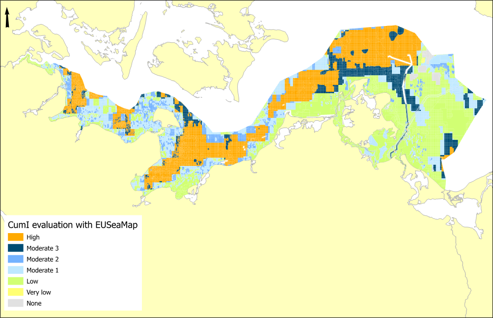
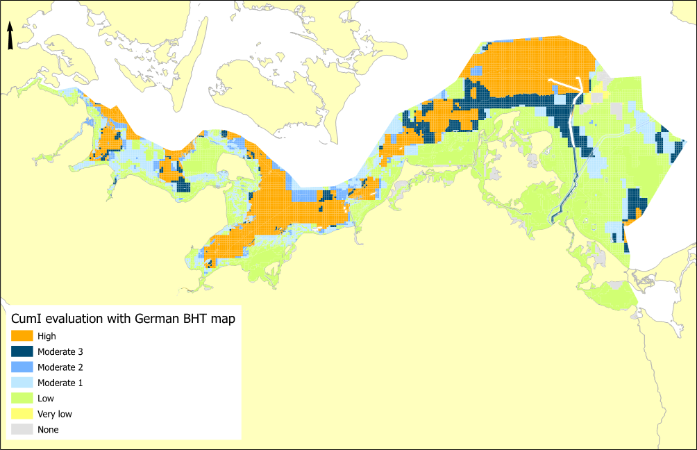
Impact evaluation result of the Cumulative impact from physical pressures on benthic biotopes indicator in the German Baltic Sea, using HELCOM data from 2016 to 2021, and benthic Broad Habitat Types according to EUSeaMap (top) and German BHT map (below). The map shows the combined potential impact from physical disturbance, including bottom trawling fishery and mariculture, extraction and disposal of sediments, platforms and wind farms, pipelines and cables, coastal protection, and shipping.
Comparing the case study result to the Baltic-wide HELCOM evaluation (see main report text), the general pattern of impact distribution is the same with respect to the individual impact classes. Highest impact is found in deeper offshore/circalittoral waters (mainly due to bottom trawling). Coastal areas and protected areas show least impact. Analysing the spatial distribution of CumI impact classes in the German Baltic Sea displays a similar extent of the cumulative physical disturbance classified as “high” and “moderate 3” in both BHT maps.
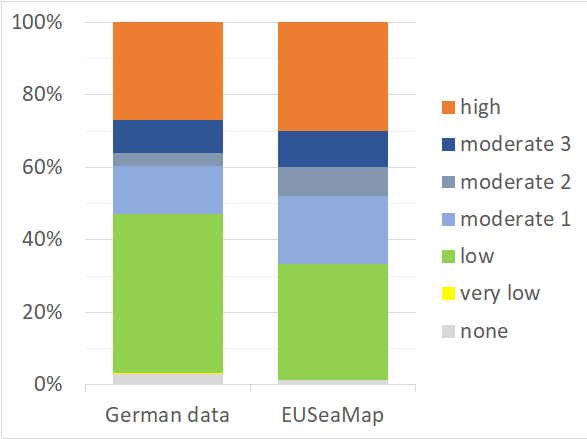
Extent percentage of potential cumulative impact (disturbance only) from physical pressures in the German Baltic Sea, based on the national German BHT map and the HELCOM EUSeaMap.
The CumI evaluation with the German BHT map shows that more than 45% of the German Baltic seafloor meet the quality threshold (impact below the m1 level of moderate impact), compared to less than 35% of the assessed area when executing the evaluation with the EUSeaMap. Even considering that the German BHT map covers a larger surface area (see explanation under Appendix B section “biotope map”), the low category (green colour) is more widely represented in the German BHT map and can be explained by the assignment to different BHTs associated with a lower sensitivity towards bottom trawling.
The results of the test case show that the assessment procedure is applicable in general. Using a different biotope map is easily done. The results in this case show a much more detailed map than in the Baltic-wide case. The visually seemingly similar spatial resolution compared to the HELCOM case is due to the predominant bottom trawling fishery which operates on a spatial scale that is not matching the fine resolution of the biotope map. As an example, the prediction of non-disturbed area (1 %) is most probably too low. The data for the pressures often does not have a fine enough spatial resolution (especially the data for bottom trawling fishery) so the disturbance percentage is overestimated. Further refinements will also be beneficial in the pressure-specific sensitivity classification. This will improve the confidence of the resulting magnitude of pressure and its potential impact.
A case study has been carried out in Swedish waters in 2020 to test the indicator concept and its applicability under local conditions. Preliminary results were presented during the online EN BENTHIC WS1-2020 Meeting in March 2020. The test evaluation showed that the indicator concept was in principle applicable. However, a detailed description is not yet included in this report as data checks and verification of the assessment results are pending.
Based on available data of several pressures in two Swedish coastal areas and sensitivity estimations from literature, evaluation results in terms of good environmental status (GES) or not-GES status could be achieved with information on the area of sea floor (km2) not affected, low or adversely affected by physical pressures. In the investigated sites, eelgrass (Swedish west coast) and vascular plants (around the coast of Blekinge and northeast Scania) were taken into account. It was not possible to assign these areas to BHTs in all cases. Further, a separation of the different substrates was not done. Some adjustments to the assessment procedure were necessary as a combined pressure layer was used for this case study (Törnqvist et al., 2019). Thus, the matrix calculation with the CumI method was started at the level of impact calculation by intersecting the magnitude of pressures with the biotope sensitivities. The impact matrix was modified based on four pressure classes and two different sensitivity classes for eelgrass at the Swedish west coast. As GES threshold for the classification of the environmental status, the present proposal of less than 25 % significantly impacted biotope area (moderate or higher impacts) and 10 % permanently not impacted biotope area was used. The evaluation was carried out at the level of individual WFD water bodies which were summed up for the total area for sand and soft substrate at the Swedish Skagerrak coast.
The following table of buffer distances is the agreed HELCOM standard set of values. These values should be regarded as default values when no other, more specific, information is available. When more specific values are available, especially those based on data or national agreements, these should be used instead for the respective area of applicability.
The numbers in the table describe the radius in metres of the buffer constructed around the pressure source and thus define the buffer zone with the pressure intensity that is indicated in the column header. A distance of 0 means that the respective zone is not constructed. The zones begin where the previous inner zone end and extend to the given radius, measured from the centre (point or line data) or the boundary (polygon data) of the pressure.
As an example, a buffer distance of 50 for a high intensity means a buffer from 0–50 metres around a pressure source. A subsequent moderate intensity of 100 then is an adjacent buffer 50–100 metres around a pressure source. So, the number in a specific columns is always the radius of the outer border of a zone, not its width.
The second column of the table lists whether there is a buffer zone counting as ‘loss’ and the last column describes whether the pressure footprint itself (in case of polygon data) is treated as loss (footprint as loss: 1 = yes, 0 = no).
| Pressure layer | loss | high | moderate | low | Very low | Footprint as loss |
| sand and gravel extraction | 0.0 | 50.0 | 100.0 | 250.0 | 500.0 | 1 |
| deposit of dredged material | 0.0 | 50.0 | 100.0 | 250.0 | 500.0 | 0 |
| maintenance dredging | 0.0 | 50.0 | 100.0 | 250.0 | 500.0 | 0 |
| capital dredging, areas | 0.0 | 0.0 | 0.0 | 0.0 | 0.0 | 1 |
| Capital dredging, points, volume ≤ 5.000 m3 | 25.0 | 25.0 | 25.0 | 25.0 | 25.0 | 1 |
| Capital dredging, points, volume > 5000 m3 | 50.0 | 50.0 | 50.0 | 50.0 | 50.0 | 1 |
| Cables under construction | 0.0 | 0.0 | 550.0 | 600.0 | 1000.0 | 0 |
| Cables in operation | 1.5 | 1.5 | 1.5 | 1.5 | 1.5 | 0 |
| pipelines under construction | 0.0 | 0.0 | 550.0 | 600.0 | 1000.0 | 1 |
| pipelines in operation | 15.0 | 15.0 | 15.0 | 90.0 | 315.0 | 0 |
| platforms under construction | 0.0 | 0.0 | 550.0 | 600.0 | 1000.0 | 0 |
| platforms in operation | 25.0 | 25.0 | 25.0 | 25.0 | 25.0 | 0 |
| offshore wind farms under construction | 0.0 | 0.0 | 550.0 | 600.0 | 1000.0 | 0 |
| offshore wind farms in operation | 30.0 | 30.0 | 40.0 | 50.0 | 130.0 | 0 |
| offshore wind farm monopile turbines in operation | 30.0 | 30.0 | 40.0 | 50.0 | 130.0 | 1 |
| coastal defence under construction | 0.0 | 50.0 | 100.0 | 250.0 | 500.0 | 0 |
| coastal defense in operation | 50.0 | 50.0 | 50.0 | 50.0 | 50.0 | 0 |
| mariculture | 150.0 | 150.0 | 400.0 | 650.0 | 1150.0 | 1 |
| harbour in operation | 200.0 | 0.0 | 0.0 | 0.0 | 0.0 | 0 |
The following table is an annotated version of the table above. It is provided as an additional source of information only. The last column informs about the source of the buffer models. (When there are deviations in the numbers between the two tables, the above table is the one used for the calculations).
Physical disturbance
| Activity/Pressure | Applied buffer * | Data processing | Remarks/Reference |
| Fishing intensity | – | swept area ratio (SAR) in ICES C-squares, surface and subsurface are considered separately | surface and subsurface SAR are used in contrast to HELCOM BSII where only subsurface was considered |
| Extraction of sand and gravel | 500 m with sharp decline | Customized buffer model (starting beyond area of loss) | HELCOM BSII
(no additional buffering in the CumI assessment if the exact removal area is known and if it is not located at the marginal zone of the polygon) |
| Deposit of dredged material | 500 m with sharp decline | Buffer for point and polygon data
Customized buffer model 50 m high |
HELCOM (EN DREDS) |
| Maintenance dredging | 500 m with sharp decline | Buffer for point and polygon data
Customized buffer model 50 m high |
HELCOM (EN DREDS) |
| Cable under construction | 1 km with sharp decline after 500 m | Customized buffer model
550 m moderate |
HELCOM BSII |
| Pipelines under construction | 1 km with sharp decline after 500 m | Customized buffer model
550 m moderate |
HELCOM BSII |
| Platforms under construction | 1 km with sharp decline after 500 m | Customized buffer model
550 m moderate |
HELCOM BSII |
| Wind farms under construction | 1 km with sharp decline after 500 m | Customized buffer model
550 m moderate |
HELCOM BSII |
| Wind farms in operation | 100 m with sharp decline | Customized buffer model (starting beyond area of loss)
10 m moderate |
HELCOM, OSPAR, Eastwood 2007, Rees 2006 |
| Pipelines in operation | 300 m with linear decline | Customized buffer model (starting beyond area of loss)
75 m low |
HELCOM BSII |
| Coastal defence under construction | 500 m with sharp decline | Customized buffer model
50 m high |
HELCOM BSII |
| Shipping | – | water depth dependent: > 0 m and ≤ 10 m (100 % intensity)> 10 m and ≤ 15 m (50 % intensity)> 15 m and ≤ 20 m (25 % intensity)> 20 m and ≤ 25 m (10 % intensity) |
HELCOM BSII |
| Mariculture | 1 km with linear decline | Customized buffer model (starting beyond area of loss)
250 m moderate |
HELCOM BSII |
*buffer used as radius, resulting spatial extent (= diameter) twice as large
Physical loss
| Activity/Pressure | Applied buffer * | Data processing | Remarks/Reference |
| Extraction of sand and gravel | – | Area of polygon, no actual extraction areas available | HELCOM BSII |
| Capital dredging | 25 m < 5000 m3
50 m > 5000 m3 |
Buffer depends on the amount dredged | HELCOM (EN DREDS) |
| Wind farms in operation | 30 m | Buffer around single turbines | Based on Foden et al. (2011) |
| Cable in operation | 1.5 m | Line data | HELCOM (German BalticBOOST case study) |
| Platforms in operation | 25 m | Point data | Exact dimensions if available |
| Pipelines in operation | 15 m | Line data | Exact dimensions if available |
| Coastal defence | 50 m | Line data | HELCOM, van der Wal & Tamis 2014 |
| Harbours | 200 m | Polygon | HELCOM, Orviku 2008 |
*buffer used as radius, resulting spatial extent (= diameter) twice as large
As estimated by ICES WKFBI (2016): Baltic broad scale habitats revised, with assigned sensitivity scores low, moderate and high. The confidence is classified as low by ICES and is mainly based on expert judgement. These sensitivities is one of the data source used for deriving the final biotope sensitivities used in the CumI (see Appendix G).
| ICES WKFBI (2016) Baltic revised sensitivities
Broadscale Habitats |
Pressure -> | Penetration and/or disturbance of the substrate below the surface of the seabed (> 2 cm) | Shallow abrasion/ penetration: damage to seabed surface and penetration (< 2 cm) |
Characteristic species (justification) | |
| A5.13: Infralittoral coarse sediment | Oligohaline | Subtidal coarse sediment | L | M | Oligochaetes, Gammarus spp., Chironomids, Macoma balthica |
| Mesohaline | L | L | Ophelia, Travisia, Mya arenaria, Macoma balthica, Cerastoderma | ||
| Polyhaline | L | H | Astarte spp., Macoma calcarea, Mya truncata, (Arctica islandica) | ||
| A5.14: Circalittoral coarse sediment | Oligohaline | Subtidal coarse sediment | L | M | Oligochaetes, Chironomids, Monoporeia affinis, Gammarus spp., Macoma balthica |
| Mesohaline | L | L | Ophelia, Travisia, Mya arenaria, Macoma balthica, Cerastoderma | ||
| Polyhaline | L | H | Astarte spp., Macoma calcarea, Mya truncata, (Arctica islandica) | ||
| A5.15: Deep Circalittoral coarse sediment | Mesohaline | Subtidal coarse sediment (> 50 m) | |||
| Polyhaline | NA | NA | |||
| A5.23: Infralittoral fine sand or A5.24: Infralittoral muddy sand | Oligohaline | Subtidal sand | M | M | Macoma balthica, Oligochaetes, Chironomids |
| Mesohaline | M | M | Mya arenaria, Macoma balthica, Cerastoderma, Polychaetes | ||
| Polyhaline | M | H | Astarte borealis, Arctica islandica, Mya arenaria, Polychaetes (partly tube-building) | ||
| A5.25: Circalittoral fine sand or A5.26: Circalittoral muddy sand | Oligohaline | Subtidal sand | M | M | Macoma balthica, Monoporeia affinis, Oligochaetes |
| Mesohaline | M | M | Mya arenaria, Macoma balthica, Cerastoderma, Polychaetes | ||
| Polyhaline | M | H | Astarte borealis, Arctica islandica, Mya arenaria, Polychaetes (partly tube-building) | ||
| A5.27: Deep circalittoral sand | Marine | Subtidal sand (> 50 m) | NA | NA | |
| A5.33: Infralittoral sandy mud | Oligohaline | Subtidal mud | M | M | Macoma balthica, Oligochaetes, Chironomids, Marenzelleria |
| Mesohaline | M | M | Macoma balthica, Polychaetes, Priapulids, Monoporeia affinis, Pontoporeia femorata | ||
| Polyhaline | H | H | Arctica islandica, Ophiura albida, Polychaetes | ||
| A5.34: Infralittoral fine mud | Oligohaline | Subtidal mud | M | M | Macoma balthica, Oligochaetes, Chironomids, Marenzelleria |
| Mesohaline | M | M | Macoma balthica, Polychaetes, Priapulids, Monoporeia affinis, Pontoporeia femorata | ||
| Polyhaline | H | H | Arctica islandica, Ophiura albida, Polychaetes | ||
| A5.35: Circalittoral sandy mud | Oligohaline | Subtidal mud | M | M | Monoporeia affinis, Saduria entomon, Macoma balthica, Marenzelleria |
| Mesohaline | M | M | Macoma balthica, Polychaetes, Priapulids, Monoporeia affinis, Pontoporeia femorata | ||
| Polyhaline | H | H | Arctica islandica, Ophiura albida, Polychaetes | ||
| A5.36: Circalittoral fine mud | Oligohaline | Subtidal mud | M | M | Monoporeia affinis, Saduria entomon, Macoma balthica, Marenzelleria |
| Mesohaline | M | M | Macoma balthica, Polychaetes, Priapulids, Monoporeia affinis, Pontoporeia femorata | ||
| Polyhaline | H | H | Arctica islandica, Ophiura albida, Polychaetes | ||
| A5.37: Deep circalittoral mud | Oligohaline | Subtidal mud (>50m) | M | M | Monoporeia affinis, Saduria entomon, Marenzelleria |
| Mesohaline | NA | NA | |||
| Polyhaline | NA | NA | |||
| A5.43: Infralittoral mixed sediments | Oligohaline | Subtidal mixed sediments | M | M | Macoma balthica, Oligochaetes, Chironomids, Marenzelleria |
| Mesohaline | L | L | Ophelia, Travisia, Mya arenaria, Macoma balthica, Cerastoderma | ||
| Polyhaline | L | H | Astarte spp., Macoma calcarea, Mya truncata, (Arctica islandica) | ||
| A5.44: Circalittoral mixed sediments | Oligohaline | Subtidal mixed sediments | M | M | Monoporeia affinis, Saduria entomon, Macoma balthica, Marenzelleria |
| Mesohaline | L | L | Ophelia, Travisia, Mya arenaria, Macoma balthica, Cerastoderma | ||
| Polyhaline | L | H | Astarte spp., Macoma calcarea, Mya truncata, (Arctica islandica) | ||
| Subtidal macrophyte-dominated sediment | Subtidal macrophyte-dominated sediment | L | M | Zostera marina | |
| Subtidal biogenic reefs | Subtidal biogenic reefs | NE | NE | Mytilus spp. |
Following a request in EN-BENTHIC 4-2020 (Annex 2, topic 1.i) the compiled studies relevant to fishing pressure from the past three years based on the input from Denmark were reviewed regarding their applicability and if possible, compared to the existing literature for CumI. The evaluated literature is divided into two categories: “Precluded literature” and “Assessed literature”. Literature in the first category was mainly excluded due to data limitations and assessments which relate to dynamic sensitivities of habitats.
After thorough evaluation of the literature, several studies had to be excluded from the analysis. The main reasons are data limitations and assessments based on dynamic sensitivities of habitats. The CumI assessment relates to a static sensitivity of habitats referring to a pristine state of the benthos. Studies including detailed justification for preclusion are listed below.
Pressure
The magnitude of pressure for bottom trawling at higher resolution was investigated by several studies.
Hiddink et al. 2016
analysed different trawling intensities to achieve maximal production of a target specie in the Kattegat
- A comparison with the CumI assessment is not possible, because the study refers to a direct application to fishing management in a specific area based on a dynamic sensitivity of habitats.
Hiddink et al. 2017 and Hiddink et al. 2019
analyzed the biomass decline/species abundance decrease per trawl pass.
- For the application in the CumI assessment, the spatial and temporal resolution of SAR is too coarse to apply theoretical trawl pass decline of benthos.
Eigaard et al. 2016 and Rijnsdorp et al. 2020
investigated the gear type dependent penetration depth allowing an estimation of pressure intensity (surface and subsurface) for 14 different functional gear groups (métiers)
- The information of vessel size, gear type, and target species composition are needed at a high temporal and spatial (1×1 min) resolution. These data are not available in the CumI assessment.
Sensitivity
Based on the longevity of benthic fauna, the sensitivity of the seabed to bottom trawling can be determined by the critical trawling intensity (Tc) at which the biomass proportion of long-lived taxa is reduced to a certain level of the untrawled reference.
provide a method to estimate the sensitivity of benthic habitats based on the longevity composition of the invertebrate community. The longevity biomass composition was estimated using benthic samples collected in the North Sea and English Channel, and related sediment composition and tidal bed-shear stress. Seabed sensitivity was estimated as the critical trawling intensity (Tc) at which the biomass of long-lived taxa is reduced to a proportion of the untrawled biomass.
- Since it is uncertain whether sampling stations recovered from historic trawl activities, vulnerable taxa may have already disappeared from the study area, affecting the biomass-longevity composition of the benthic community
- Tc which is based on longevity distribution of the benthic community relates to dynamic sensitivity of habitats and therefore cannot be compared to the static sensitivity of habitats applied in the CumI assessment
Using the longevity distribution of the untrawled infaunal community, the seabed integrity was estimated as the proportion of the biomass of benthic taxa where the trawling interval at the subsurface level exceeds their life span.
analysed the seabed integrity (SBI) and the distribution and intensity of bottom trawling in European waters. SBI was estimated as the proportion of the biomass of benthic taxa where the trawling interval at the subsurface level exceeds their life span, with SBI ranging between 0 (all taxa potentially impacted) and 1 (none of the tax impacted). For calculating SBI indicator, regression parameters were based on biomass-longevity data of infaunal taxa taken from sampling stations in the North Sea with unknown trawl history. Indicators for trawling pressure were based on VMS data coupled to logbook data and analysed at a resolution of 1 x 1min longitude and latitude for different EUNIS habitat types and main gear groups. Combined with the information on target species and gear type allowed the distinction between surface and subsurface footprints.
- The SBI indicator – whose regression parameters are not based on samples taken from pristine untrawled areas- relates to dynamic sensitivity of habitats and therefore cannot be compared to the static sensitivity of habitats applied in the CumI assessment
- Furthermore, the SBI indicator ignores the possible differences in the longevity distribution of the benthic community across habitats.
Trawling intensity within small spatial area (1×1 minute longitude and latitude) bottom trawling activity can be considered as randomly distributed on an annual basis (Rijnsdorp et al. 1998, Lee et al. 2010) and is a prerequisite for the calculation of the seabed integrity (SBI).
- Calculation of different indicators for trawling pressure is not applicable in the CumI assessment, because spatial resolution of SAR is too coarse.
uses of VMS/Logbook data and applies the LL1 as well as the population dynamic (PD) methods to assess the impact of trawling relate to. The Longevity (LL1) method: statistical model – longevity composition of a benthic community tracks changes in benthic community composition in response to trawling, with 0 = no impact, 1 = maximum possible impact (Rjinsdorp et al. 2016). The indicator estimates the reduction in the proportion of long-lived taxa (maximum lifespan > 10 years) caused by trawling. The population dynamic (PD) method is a mechanistic model estimating the total reduction in the community biomass relative to carrying capacity (relative benthic status RBS) in response to trawling (gear specific depletion rates) and the recovery time (recovery rates).
- Both impact assessment methods (LL1, PD) relate to dynamic sensitivity of habitats and therefore cannot be compared to static habitat sensitivity used in the CumI assessment
- Comparison with CumI is not possible, because detailed VMS/Logbook data are not available for the CumI assessment and spatial and temporal resolution of SAR is too coarse
- no information on gear type is available to derive gear-specific depletion rates
Impact
estimated depletion rates and intrinsic recovery rates of community in response to experimental trawling. In case longevity distribution of a community is known, both parameters can be combined with high-resolution maps of trawling intensity to assess trawling impacts at the scale of the fishery or other defined unit of assessment. They apply the relative benthic status (RBS) method which is based on the longevity distribution of the present benthic community accounting for the interaction of other forms of disturbance including trawling.
- RBS method relates to dynamic habitat sensitivities and therefore cannot be compared to static sensitivities of habitats used in the CumI assessment
- Additionally, depletion and recovery rates after trawling cannot be applied in the CumI assessment because the resolution of SAR value is spatially and temporally too coarse. Neither exact trawling location nor its trawling interval between trawls are available to apply depletion rates or recovery rates of species’ community in a small spatial area.
concluded that whole-community numbers of individuals and biomass are most suitable indicators of bottom trawling impact on the state of benthic biota. The assessment of biomass decline per trawl needs to be carried out in pristine reference areas to be comparable to the magnitude of impact in the CumI assessment. But “pristine conditions” of reference areas cannot be guaranteed (see Hiddink et al. 2019)
- Comparison with Magnitude of impact of the CumI assessment is not applicable since the study relates to a dynamic sensitivity of habitats
ICES 2019a, Annex 4 – technical guidance document
The document describes the methodology of an assessment approach that can be used to derive a set of indicators for assessing physical disturbance pressures from bottom-contacting fishing gears and their environmental impacts on seabed habitats. The guidance document suggests applying the RBS method which is based on the longevity distribution of the present benthic community accounting for the interaction of other forms of disturbance including trawling.
- RBS method relates to dynamic habitat sensitivities and therefore cannot be compared to static sensitivities of habitats used in the CumI assessment (see Hiddink et al. 2019).
- Additionally, depletion and recovery rates after trawling cannot be applied in the CumI assessment because the resolution of SAR value is spatially and temporally too coarse (see Hiddink et al. 2019).
The following trawling literature was approved for comparison and details are listed below
Pressure
examined the effects of trawl and natural (tidal-bed shear stress) disturbance on benthic communities over gradients of bottom trawling effort in the North and Irish Seas. Both sources of disturbance caused declines in long-living, hard-bodied (exoskeleton) and suspension-feeding organisms, resulting in no detectable trawling effect on communities exposed to high natural disturbance. The findings will help to identify areas that are more resilient to trawling and support the development of management plans. Although the origin of their trawling categories is unclear, trawl intensity in the following SAR-categories can be compared:
| CumI intensity categories | CumI SAR ranges | Van Denderen et al. 2015 | SAR ranges |
| very low | 0.05 ≤ SAR < 0.33 | ||
| low | 0.33 ≤ SAR < 0.66 | low | SAR ≤ 0.2 |
| moderate | 0.66 ≤ SAR < 2.00 | intermediate | 0.2 < SAR ≤ 0.5 |
- SAR-categories used in CumI are less cautious compared to ranges of SAR-values used in Van Denderen et al. (2015)
Sensitivity
The biomass-longevity distribution can be used as an indicator for habitat sensitivity. The higher the proportion of long-lived taxa with low resilience (slow recovery after trawl impact), the higher the sensitivity of the habitat.
modelled the longevity distribution of the benthic community in the Baltic Sea based on biomass-longevity data and the underlying environmental conditions of depth, salinity, and wave exposure at the seabed. In the CumI assessment sensitivity distribution of biotopes are mainly based on environmental conditions such as sediment composition, salinity, depth (infra vs. circa) and characteristic species.
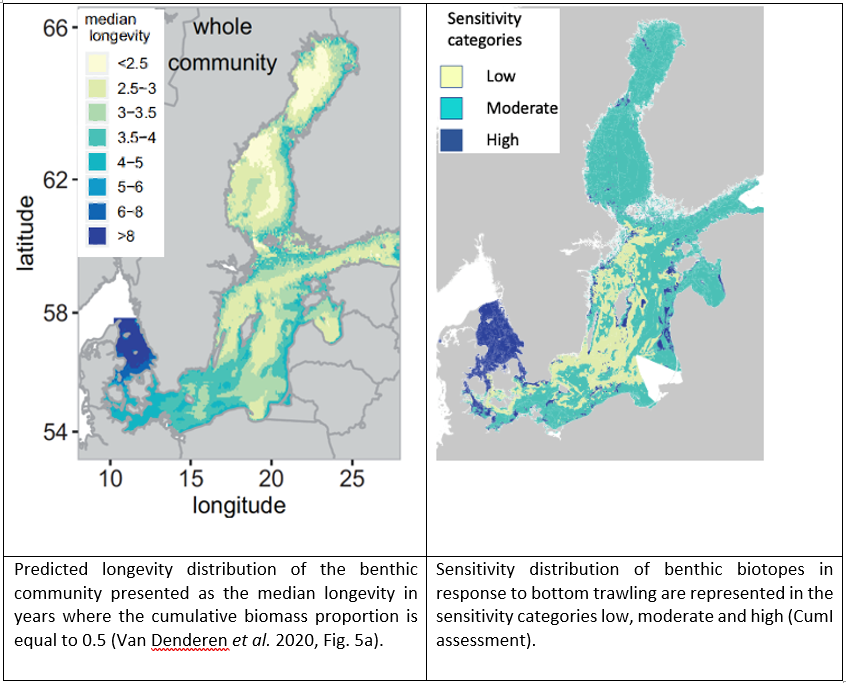
- The pattern of the longevity distribution in the Baltic is in good agreement with the sensitivity map of biotopes in response to trawling, showing highest values in the Kattegat, moderate ones in southern part of the Western Baltic and low values in the Gotland basin. Comparison will be revised after assessing completed sensitivity survey
- However, longevity distribution of the benthic community referred to as a reference state (Van Denderen et al. 2020) might be influenced by trawling, because no information on collated data is given, if samples were taken in untrawled “pristine areas” (Gogina et al. 2016). In this case, the longevity–biomass composition – displaying a dynamic population – relates to a dynamic sensitivity of habitats and a direct comparison with a static sensitivity of habitats applied in CumI is partly biased.
Life spans of characteristic species (MarLIN-database)
associated with Baltic broad scale habitats (see revised table by ICES WKFBI, 2016) are compared to the median longevity distribution in the Baltic Sea
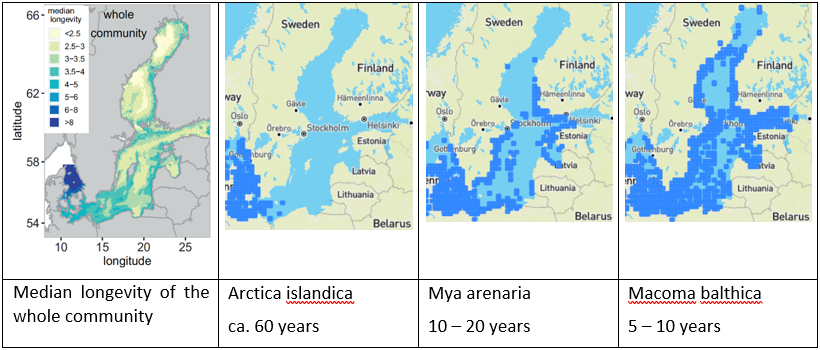 Distribution of longevity of whole community (Van Denderen et al. 2020, Fig. 5a) and distribution of characteristic species (bivalves) with associated life spans (MarLIN – https://www.marlin.ac.uk/species) in the Baltic Sea. By contributing significantly to the cumulative biomass, bivalves influence the biomass-longevity distribution and consequently the median longevity of the benthic community.
- The pattern of longevity distribution in the Baltic is in good agreement with the distribution of maximal life spans of characteristic species, displaying younger ages associated with lower salinities.
analysed available data for experimental and comparative studies of trawling impacts on whole communities of seabed macroinvertebrates in sedimentary habitats and developed a widely applicable method to estimate depletion and recovery rates of biota after trawling. Coupled with high resolution maps of trawling frequency and habitat, the RBS method enables assessment of trawling impacts on present benthic macrofaunal communities. Some of the comparative studies used for estimating recovery rates as well as of the experimental studies on depletion, were conducted in previously trawled areas with a lowered abundance of biota. This automatically results in a lowered sensitivity of habitats. Hence the RBS method relates to a dynamic sensitivity of habitats as opposed to the static sensitivity used for the CumI assessment.
Despite significant methodological differences between RBS-method and CumI assessment, we evaluated the pattern of resilience to trawling across habitats in marine waters and the Baltic Sea in relation to their rough sediment classification. For the comparison we used the revised ICES broad scale habitats (ICES WKFBI, 2016) with assigned resilience scores to shallow abrasion/penetration in polyhaline waters, being closest to full marine waters and covering a range of different sediment types.
Applying the RBS-method, habitat resilience, represented by recovery rates, is inversely correlated to gravel content. Hiddink et al. (2017) assumed that communities on gravel may be more sensitive to trawling, because they, on average, have a larger proportion of larger, long-lived, and sessile epifauna (Bolam et al. 2017) showing longer recovery times after physical disturbance. On the other hand, high recovery rates indicating high resilience of habitats, are associated with sediments lacking gravel.
The ICES broad scale habitats characterized by coarse sediments show low resilience to abrasion like the response of habitats with high gravel content (RBS-method). In contrast to the resilience pattern based on the RBS-method, the Baltic broad scale habitats with subtidal mud and sand (no gravel) show very low resilience to abrasion.
- Pattern of sediment-depended resilience of habitats according to RBS-method does not match ICES pattern, displaying very low or low habitat resilience irrespective of gravel content
For assessing sensitivities of Baltic broad scale habitats, ICES assigned characteristic species and their responses to different pressures to habitats. A characteristic specie of these habitats is Arctica islandica, a long-lived bivalve with low recovery rates leading to very low resilience to physical abrasion. This specie is also spread in the Northwest and northeast Atlantic (MarLIN database) matching areas of evaluated studies with unknown trawling history for developing the RBS-method. Arctica islandica as well as other long-lived biota sensitive to trawling, might be significantly depleted, thus contributing little to the recovery rate of the whole community.
- As a result, the RBS-method most likely overestimates average recovery rate and thus resilience to trawling of the benthic community, while the CumI assessment relates to static resilience of habitats in pristine conditions.
Estimating the sustainability of towed fishing-gear impacts on seabed habitats: a simple quantitative risk assessment method applicable to data-limited fisheries. The applied RBS-method relates to dynamic sensitivity of habitats: caution when comparing to static habitat sensitivity in CumI assessment (see Hiddink et al. 2017)
Habitat sensitivity is dependent on resistance which can be represented by biomass /abundance depletion per trawl pass. Pitcher et al. 2017 assessed that habitat dependent depletion is highest in habitats associated with gravel.
This result is in line with habitat sensitivity in the CumI assessment showing high sensitivities to shallow abrasion in habitats associated with hard substrate throughout all countries. Habitats characterized with sand, mud or mixed sediments potentially have lower sensitivities. However, comparison with biotope sensitivities to trawling will be reassessed after evaluating results of the sensitivity survey.
Eigaard et al. 2017
SBI – seabed integrity was estimated as the proportion of the biomass of benthic taxa where the trawling interval at the subsurface level exceeds their life span, with seabed integrity indicator (SBI) ranging between 0 (all taxa potentially impacted) and 1 (none of the tax impacted) to estimate critical trawling intensity (Tc).
The constants/parameters for calculating SBI are based on biomass-longevity data of infaunal taxa taken from sampling stations with unknown trawling history.
- SBI-calculations relate to a dynamic sensitivity. At an annual trawling intensity of 0.1 year-1 to be a critical intensity beyond which bottom trawling may start compromising the integrity of the seabed and associated benthic community. This critical intensity was based on the data from van Denderen et al. (2015) showing that about 17% of the infaunal biomass comprised of taxa with longevity of 10 years or more. The critical trawling intensity based on the longevity composition can be considered to be a low-risk reference. It does not mean that taxa that are trawled at least once during their lifespan will no longer be able to maintain themselves.
| CumI intensity categories | CumI SAR ranges |
| very low | 0.05 ≤ SAR < 0.33 |
| low | 0.33 ≤ SAR < 0.66 |
- CumI follows a less cautious approach
Sciberras et al. 2018
investigated the response of benthic fauna to experimental bottom fishing. Pressure sensitivities of characteristic species in Baltic broad scale habitats (ICES WKFBI, 2016) were analysed according to MarLIN and results compared to the corresponding taxonomic classes in the study of Sciberras et al. 2018.
An evaluation of both sensitivity patterns is not possible because sensitivities of single species to surface abrasion are compared with average sensitivities of a whole taxonic groups. Furthermore, characteristic species of broad scale habitats in the Baltic Sea cover only 4 of 13 taxonomic classes described in Sciberras et al. 2018
However, if habitat characteristic species are assigned to taxonomic classes following statements can be made: all characteristic species show a low or medium resistance to abrasion indicating that they are affected by a trawl pass.
- This is in line with the results of the study (Sciberras et al. 2018) demonstrating that the corresponding taxonomic classes (Bivalvia, Polychaeta, Clitellata and Malacostraca) show a significant depletion per gear pass (Sciberras et al. 2018, Fig. 7).
Furthermore, most characteristic species show a high resilience to abrasion, describing the recoverability after trawling (except bivalve Arctica islandica). This coincides with positive recovery rates of the corresponding taxonomic classes resulting in recovery times of 1 to 7 months after a gear pass (Sciberras et al. 2018, Tab. 3).
The following table lists the sensitivity categories used for the evaluation, divided into the relevant member states, MSFD broad scale habitats (BHT) and salinity range.
The current values are a result of the agreed values from the final CumI test run and documented in the CumI report version from 2021-09-07 (in case of erroneous multiple assignments for the same biotope/salinity combination, the value covering the larger area in the last evaluation was taken). Sensitivity values of country/biotope/salinity combinations not yet assigned but necessary due to the new EUSeaMap from September 2021 and updated salinity map were preferably taken from the adjacent salinity class within the same country/biotope combination. The short names for the BHTs used here are mapped to the full names as follows:
- “Circalittoral rock and biogenic reef” = “circa hard”
- “Circalittoral coarse sediment” = “circa hard”
- “Circalittoral mixed sediment” = “circa mix”
- “Circalittoral mud” = “circa mud”
- “Circalittoral sand” = “circa sand”
- “Infralittoral rock and biogenic reef” = “infra hard”
- “Infralittoral coarse sediment” = “infra hard”
- “Infralittoral mixed sediment” = “infra mix”
- “Infralittoral mud” = “infra mud”
- “Infralittoral sand” = “infra sand”
- “Offshore circalittoral coarse sediment” = “circa hard”
- “Offshore circalittoral mixed sediment” = “circa mix”
- “Offshore circalittoral mud” = “circa mud”
- “Offshore circalittoral rock and biogenic reef” = “circa hard”
- “Offshore circalittoral sand” = “circa sand”
In the EUSeaMap, some BHT are a “combination” of two basic BHT. This is true for “Circalittoral mud or Circalittoral sand”, “Infralittoral mud or Infralittoral sand” and “Offshore circalittoral mud or Offshore circalittoral sand”. These are mapped to the most sensitive of the two basic BHTs and the sensitivity is assigned accordingly. All “offshore” BHT are treated as the corresponding BHT in the circalittoral zone.
| Territory | MSFD BHT | Salinity range (psu) | General sensitivity | Bottom trawling sensitivity |
|---|---|---|---|---|
| Denmark | circa hard | 7.5-11 | high | high |
| Denmark | circa hard | 11-18 | high | high |
| Denmark | circa hard | 18-30 | high | high |
| Denmark | circa hard | > 30 | high | high |
| Denmark | circa mix | 7.5-11 | high | low |
| Denmark | circa mix | 11-18 | high | low |
| Denmark | circa mix | 18-30 | high | low |
| Denmark | circa mix | > 30 | high | low |
| Denmark | circa mud | 7.5-11 | moderate | moderate |
| Denmark | circa mud | 11-18 | moderate | moderate |
| Denmark | circa mud | 18-30 | moderate | high |
| Denmark | circa mud | > 30 | moderate | high |
| Denmark | circa sand | 7.5-11 | low | moderate |
| Denmark | circa sand | 11-18 | low | moderate |
| Denmark | circa sand | 18-30 | low | high |
| Denmark | circa sand | > 30 | low | high |
| Denmark | infra hard | 7.5-11 | high | high |
| Denmark | infra hard | 11-18 | high | high |
| Denmark | infra hard | 18-30 | high | high |
| Denmark | infra hard | > 30 | high | high |
| Denmark | infra mix | 7.5-11 | high | low |
| Denmark | infra mix | 11-18 | high | low |
| Denmark | infra mix | 18-30 | high | high |
| Denmark | infra mix | > 30 | high | high |
| Denmark | infra mud | 7.5-11 | moderate | moderate |
| Denmark | infra mud | 11-18 | moderate | moderate |
| Denmark | infra mud | 18-30 | moderate | high |
| Denmark | infra mud | > 30 | moderate | high |
| Denmark | infra sand | 7.5-11 | low | moderate |
| Denmark | infra sand | 11-18 | low | moderate |
| Denmark | infra sand | 18-30 | low | high |
| Denmark | infra sand | > 30 | low | high |
| Estonia | circa hard | 5-7.5 | high | high |
| Estonia | circa hard | 7.5-11 | high | high |
| Estonia | circa mix | 5-7.5 | moderate | high |
| Estonia | circa mix | 7.5-11 | moderate | low |
| Estonia | circa mud | 5-7.5 | moderate | moderate |
| Estonia | circa mud | 7.5-11 | moderate | moderate |
| Estonia | circa sand | 5-7.5 | moderate | moderate |
| Estonia | circa sand | 7.5-11 | moderate | moderate |
| Estonia | infra hard | 5-7.5 | high | high |
| Estonia | infra hard | 7.5-11 | high | high |
| Estonia | infra mix | 5-7.5 | moderate | moderate |
| Estonia | infra mix | 7.5-11 | moderate | moderate |
| Estonia | infra mud | 5-7.5 | moderate | moderate |
| Estonia | infra mud | 7.5-11 | moderate | moderate |
| Estonia | infra sand | 5-7.5 | moderate | moderate |
| Estonia | infra sand | 7.5-11 | moderate | moderate |
| Finland | circa hard | < 5 | high | high |
| Finland | circa hard | 5-7.5 | high | high |
| Finland | circa hard | 7.5-11 | high | high |
| Finland | circa mix | < 5 | moderate | moderate |
| Finland | circa mix | 5-7.5 | moderate | moderate |
| Finland | circa mix | 7.5-11 | moderate | moderate |
| Finland | circa mud | < 5 | moderate | moderate |
| Finland | circa mud | 5-7.5 | moderate | moderate |
| Finland | circa mud | 7.5-11 | moderate | moderate |
| Finland | circa sand | < 5 | moderate | moderate |
| Finland | circa sand | 5-7.5 | moderate | moderate |
| Finland | circa sand | 7.5-11 | moderate | moderate |
| Finland | infra hard | < 5 | high | high |
| Finland | infra hard | 5-7.5 | high | high |
| Finland | infra hard | 7.5-11 | high | high |
| Finland | infra mix | < 5 | moderate | moderate |
| Finland | infra mix | 5-7.5 | moderate | moderate |
| Finland | infra mix | 7.5-11 | moderate | moderate |
| Finland | infra mud | < 5 | moderate | moderate |
| Finland | infra mud | 5-7.5 | moderate | moderate |
| Finland | infra mud | 7.5-11 | moderate | moderate |
| Finland | infra sand | < 5 | moderate | moderate |
| Finland | infra sand | 5-7.5 | moderate | moderate |
| Finland | infra sand | 7.5-11 | moderate | moderate |
| Germany | circa hard | 5-7.5 | high | high |
| Germany | circa hard | 7.5-11 | high | high |
| Germany | circa hard | 11-18 | high | high |
| Germany | circa hard | 18-30 | high | high |
| Germany | circa mix | 5-7.5 | moderate | low |
| Germany | circa mix | 7.5-11 | moderate | low |
| Germany | circa mix | 11-18 | moderate | high |
| Germany | circa mix | 18-30 | moderate | high |
| Germany | circa mud | 5-7.5 | moderate | moderate |
| Germany | circa mud | 7.5-11 | moderate | moderate |
| Germany | circa mud | 11-18 | moderate | high |
| Germany | circa mud | 18-30 | moderate | high |
| Germany | circa sand | 5-7.5 | moderate | moderate |
| Germany | circa sand | 7.5-11 | moderate | moderate |
| Germany | circa sand | 11-18 | moderate | moderate |
| Germany | circa sand | 18-30 | moderate | moderate |
| Germany | infra hard | 5-7.5 | high | high |
| Germany | infra hard | 7.5-11 | high | high |
| Germany | infra hard | 11-18 | high | high |
| Germany | infra hard | 18-30 | high | high |
| Germany | infra mix | 5-7.5 | moderate | moderate |
| Germany | infra mix | 7.5-11 | moderate | low |
| Germany | infra mix | 11-18 | moderate | low |
| Germany | infra mix | 18-30 | moderate | high |
| Germany | infra mud | 5-7.5 | moderate | moderate |
| Germany | infra mud | 7.5-11 | moderate | moderate |
| Germany | infra mud | 11-18 | moderate | moderate |
| Germany | infra mud | 18-30 | moderate | high |
| Germany | infra sand | 5-7.5 | moderate | moderate |
| Germany | infra sand | 7.5-11 | moderate | moderate |
| Germany | infra sand | 11-18 | moderate | high |
| Germany | infra sand | 18-30 | moderate | high |
| Latvia | circa hard | < 5 | high | high |
| Latvia | circa hard | 5-7.5 | high | high |
| Latvia | circa hard | 7.5-11 | high | high |
| Latvia | circa hard | 11-18 | high | high |
| Latvia | circa mix | 5-7.5 | moderate | low |
| Latvia | circa mix | 7.5-11 | moderate | low |
| Latvia | circa mix | 11-18 | moderate | low |
| Latvia | circa mud | < 5 | moderate | moderate |
| Latvia | circa mud | 5-7.5 | moderate | moderate |
| Latvia | circa mud | 7.5-11 | moderate | moderate |
| Latvia | circa mud | 11-18 | moderate | moderate |
| Latvia | circa sand | < 5 | moderate | moderate |
| Latvia | circa sand | 5-7.5 | moderate | moderate |
| Latvia | circa sand | 7.5-11 | moderate | moderate |
| Latvia | circa sand | 11-18 | moderate | moderate |
| Latvia | infra hard | < 5 | high | high |
| Latvia | infra hard | 5-7.5 | high | high |
| Latvia | infra hard | 7.5-11 | high | high |
| Latvia | infra hard | 11-18 | high | high |
| Latvia | infra mix | < 5 | moderate | moderate |
| Latvia | infra mix | 5-7.5 | moderate | moderate |
| Latvia | infra mix | 7.5-11 | moderate | moderate |
| Latvia | infra mix | 11-18 | moderate | moderate |
| Latvia | infra mud | < 5 | moderate | moderate |
| Latvia | infra mud | 5-7.5 | moderate | moderate |
| Latvia | infra mud | 7.5-11 | moderate | moderate |
| Latvia | infra mud | 11-18 | moderate | moderate |
| Latvia | infra sand | < 5 | moderate | moderate |
| Latvia | infra sand | 5-7.5 | moderate | moderate |
| Latvia | infra sand | 7.5-11 | moderate | moderate |
| Latvia | infra sand | 11-18 | moderate | moderate |
| Lithuania | circa hard | 5-7.5 | high | high |
| Lithuania | circa hard | 7.5-11 | high | high |
| Lithuania | circa mix | 5-7.5 | moderate | low |
| Lithuania | circa mix | 7.5-11 | moderate | low |
| Lithuania | circa mix | 11-18 | moderate | low |
| Lithuania | circa mud | 5-7.5 | moderate | moderate |
| Lithuania | circa mud | 7.5-11 | moderate | moderate |
| Lithuania | circa sand | < 5 | moderate | moderate |
| Lithuania | circa sand | 5-7.5 | moderate | moderate |
| Lithuania | circa sand | 7.5-11 | moderate | moderate |
| Lithuania | infra hard | < 5 | high | high |
| Lithuania | infra hard | 5-7.5 | high | high |
| Lithuania | infra hard | 7.5-11 | high | high |
| Lithuania | infra mix | 5-7.5 | moderate | moderate |
| Lithuania | infra mix | 7.5-11 | moderate | moderate |
| Lithuania | infra mud | 5-7.5 | moderate | moderate |
| Lithuania | infra mud | 7.5-11 | moderate | moderate |
| Lithuania | infra sand | 5-7.5 | moderate | moderate |
| Lithuania | infra sand | 7.5-11 | moderate | moderate |
| Poland | circa hard | 5-7.5 | high | high |
| Poland | circa hard | 7.5-11 | high | high |
| Poland | circa hard | 11-18 | high | high |
| Poland | circa mix | 5-7.5 | moderate | moderate |
| Poland | circa mix | 7.5-11 | moderate | moderate |
| Poland | circa mix | 11-18 | moderate | moderate |
| Poland | circa mud | < 5 | moderate | moderate |
| Poland | circa mud | 5-7.5 | moderate | moderate |
| Poland | circa mud | 7.5-11 | moderate | moderate |
| Poland | circa mud | 11-18 | moderate | moderate |
| Poland | circa sand | < 5 | moderate | moderate |
| Poland | circa sand | 5-7.5 | moderate | moderate |
| Poland | circa sand | 7.5-11 | moderate | moderate |
| Poland | circa sand | 11-18 | moderate | moderate |
| Poland | infra hard | 5-7.5 | high | high |
| Poland | infra hard | 7.5-11 | high | high |
| Poland | infra hard | 11-18 | high | high |
| Poland | infra mix | < 5 | moderate | moderate |
| Poland | infra mix | 5-7.5 | moderate | moderate |
| Poland | infra mix | 7.5-11 | moderate | moderate |
| Poland | infra mud | < 5 | moderate | moderate |
| Poland | infra mud | 5-7.5 | moderate | moderate |
| Poland | infra mud | 7.5-11 | moderate | moderate |
| Poland | infra mud | 11-18 | moderate | moderate |
| Poland | infra sand | < 5 | moderate | moderate |
| Poland | infra sand | 5-7.5 | moderate | moderate |
| Poland | infra sand | 7.5-11 | moderate | moderate |
| Poland | infra sand | 11-18 | moderate | moderate |
| Russia | circa hard | < 5 | moderate | moderate |
| Russia | circa hard | 5-7.5 | moderate | moderate |
| Russia | circa hard | 7.5-11 | moderate | moderate |
| Russia | circa hard | 11-18 | moderate | moderate |
| Russia | circa mix | < 5 | moderate | moderate |
| Russia | circa mix | 5-7.5 | moderate | moderate |
| Russia | circa mix | 7.5-11 | moderate | moderate |
| Russia | circa mix | 11-18 | moderate | moderate |
| Russia | circa mud | < 5 | moderate | moderate |
| Russia | circa mud | 5-7.5 | moderate | moderate |
| Russia | circa mud | 7.5-11 | moderate | moderate |
| Russia | circa mud | 11-18 | moderate | moderate |
| Russia | circa sand | < 5 | moderate | moderate |
| Russia | circa sand | 5-7.5 | moderate | moderate |
| Russia | circa sand | 7.5-11 | moderate | moderate |
| Russia | circa sand | 11-18 | moderate | moderate |
| Russia | infra hard | < 5 | moderate | moderate |
| Russia | infra hard | 5-7.5 | moderate | moderate |
| Russia | infra hard | 7.5-11 | moderate | moderate |
| Russia | infra hard | 11-18 | moderate | moderate |
| Russia | infra mix | < 5 | moderate | moderate |
| Russia | infra mix | 5-7.5 | moderate | moderate |
| Russia | infra mix | 7.5-11 | moderate | moderate |
| Russia | infra mix | 11-18 | moderate | moderate |
| Russia | infra mud | < 5 | moderate | moderate |
| Russia | infra mud | 5-7.5 | moderate | moderate |
| Russia | infra mud | 7.5-11 | moderate | moderate |
| Russia | infra mud | 11-18 | moderate | moderate |
| Russia | infra sand | < 5 | moderate | moderate |
| Russia | infra sand | 5-7.5 | moderate | moderate |
| Russia | infra sand | 7.5-11 | moderate | moderate |
| Russia | infra sand | 11-18 | moderate | moderate |
| Sweden | circa hard | < 5 | high | low |
| Sweden | circa hard | 5-7.5 | high | high |
| Sweden | circa hard | 7.5-11 | high | high |
| Sweden | circa hard | 11-18 | high | high |
| Sweden | circa hard | 18-30 | high | high |
| Sweden | circa hard | > 30 | high | high |
| Sweden | circa mix | < 5 | moderate | low |
| Sweden | circa mix | 5-7.5 | moderate | low |
| Sweden | circa mix | 7.5-11 | moderate | moderate |
| Sweden | circa mix | 11-18 | moderate | moderate |
| Sweden | circa mix | 18-30 | moderate | high |
| Sweden | circa mix | > 30 | moderate | moderate |
| Sweden | circa mud | < 5 | moderate | low |
| Sweden | circa mud | 5-7.5 | moderate | moderate |
| Sweden | circa mud | 7.5-11 | moderate | moderate |
| Sweden | circa mud | 11-18 | moderate | moderate |
| Sweden | circa mud | 18-30 | moderate | high |
| Sweden | circa mud | > 30 | moderate | high |
| Sweden | circa sand | < 5 | moderate | low |
| Sweden | circa sand | 5-7.5 | moderate | moderate |
| Sweden | circa sand | 7.5-11 | moderate | moderate |
| Sweden | circa sand | 11-18 | moderate | moderate |
| Sweden | circa sand | 18-30 | moderate | high |
| Sweden | circa sand | > 30 | moderate | high |
| Sweden | infra hard | < 5 | high | low |
| Sweden | infra hard | 5-7.5 | high | moderate |
| Sweden | infra hard | 7.5-11 | high | high |
| Sweden | infra hard | 11-18 | high | high |
| Sweden | infra hard | 18-30 | high | high |
| Sweden | infra hard | > 30 | high | high |
| Sweden | infra mix | < 5 | moderate | low |
| Sweden | infra mix | 5-7.5 | moderate | moderate |
| Sweden | infra mix | 7.5-11 | moderate | moderate |
| Sweden | infra mix | 11-18 | moderate | high |
| Sweden | infra mix | 18-30 | moderate | high |
| Sweden | infra mix | > 30 | moderate | high |
| Sweden | infra mud | < 5 | moderate | low |
| Sweden | infra mud | 5-7.5 | moderate | moderate |
| Sweden | infra mud | 7.5-11 | moderate | moderate |
| Sweden | infra mud | 11-18 | moderate | high |
| Sweden | infra mud | 18-30 | moderate | high |
| Sweden | infra mud | > 30 | moderate | high |
| Sweden | infra sand | < 5 | moderate | low |
| Sweden | infra sand | 5-7.5 | moderate | moderate |
| Sweden | infra sand | 7.5-11 | moderate | moderate |
| Sweden | infra sand | 11-18 | moderate | moderate |
| Sweden | infra sand | 18-30 | moderate | moderate |
| Sweden | infra sand | > 30 | moderate | high |
Evaluation results of the Cumulative impact from physical pressures on benthic biotopes on a Baltic-wide scale. The tables show the percentage (area) of the individual broad habitat types potentially disturbed and the corresponding disturbance category (m1, m2 and m3 are three different grades of moderate disturbance, the category “none/n.a.” represents unaffected areas (none) including areas not evaluated (n.a.) due to lack of data; delivered data do not indicate areas with lack of data). Table 29 includes the disturbance category very high which is considered as loss (very high/loss):
Table 27 Baltic Sea without loss
| Infralittoral rock and biogenic reef | Infralittoral coarse sediment | Infralittoral mixed sediment | Infralittoral sand | Infralittoral mud or Infralittoral sand | Infralittoral mud | Circalittoral rock and biogenic reef | Circalittoral coarse sediment | Circalittoral mixed sediment | Circalittoral sand | Circalittoral mud or Circalittoral sand | Circalittoral mud | Offshore circalittoral rock and biogenic reef | Offshore circalittoral coarse sediment | Offshore circalittoral mixed sediment | Offshore circalittoral sand | Offshore circalittoral mud or Offshore circalittoral sand | Offshore circalittoral mud | |
| none | 45.9 | 21.0 | 39.0 | 13.6 | 59.0 | 17.8 | 74.1 | 65.0 | 77.7 | 41.7 | 80.5 | 59.1 | 94.8 | 86.2 | 60.2 | 30.8 | 83.3 | 34.9 |
| very low | 0 | <0.1 | 0.3 | 16.0 | 0.2 | <0.1 | 0 | <0.1 | 1.6 | 4.1 | 0.1 | <0.1 | 0 | 0 | 3.1 | 0.6 | <0.1 | 0 |
| low | 6.0 | 2.1 | 9.6 | 17.8 | 16.7 | 22.3 | 3.5 | 4.3 | 9.1 | 27.1 | 13.3 | 9.5 | 0.3 | 0 | 11.9 | 15.3 | 12.4 | 11.3 |
| m1 | 44.8 | 58.7 | 45.0 | 25.7 | 23.2 | 48.2 | 21.5 | 24.6 | 10.2 | 11.1 | 4.9 | 15.4 | 1.7 | 6.4 | 5.3 | 10.2 | 2.6 | 6.7 |
| m2 | 3.2 | 16.0 | 5.1 | 15.1 | 0.7 | 9.2 | 0.9 | 4.6 | 0.6 | 3.2 | 0.3 | 2.3 | 0.8 | 1.5 | 1.0 | 1.6 | <0.1 | 0.5 |
| m3 | <0.1 | <0.1 | <0.1 | 2.8 | <0.1 | 0.6 | <0.1 | <0.1 | 0.5 | 5.9 | 0.7 | 3.0 | 0 | 0 | 8.0 | 12.1 | 1.3 | 12.7 |
| high | 0.2 | 2.1 | 1.1 | 8.9 | 0.2 | 1.8 | <0.1 | 1.5 | 0.3 | 7.0 | <0.1 | 10.6 | 2.5 | 5.9 | 10.5 | 29.4 | 0.4 | 33.9 |
Table 28 Baltic Sea with loss
| Infralittoral rock and biogenic reef | Infralittoral coarse sediment | Infralittoral mixed sediment | Infralittoral sand | Infralittoral mud or Infralittoral sand | Infralittoral mud | Circalittoral rock and biogenic reef | Circalittoral coarse sediment | Circalittoral mixed sediment | Circalittoral sand | Circalittoral mud or Circalittoral sand | Circalittoral mud | Offshore circalittoral rock and biogenic reef | Offshore circalittoral coarse sediment | Offshore circalittoral mixed sediment | Offshore circalittoral sand | Offshore circalittoral mud or Offshore circalittoral sand | Offshore circalittoral mud | |
| none | 45.7 | 21.0 | 38.9 | 13.6 | 58.9 | 17.8 | 74.0 | 64.9 | 77.7 | 41.6 | 80.5 | 59.1 | 94.8 | 86.2 | 60.1 | 30.8 | 83.2 | 34.8 |
| very low | 0 | <0.1 | 0.3 | 16.0 | 0.2 | <0.1 | 0 | <0.1 | 1.6 | 4.0 | 0.1 | <0.1 | 0 | 0 | 3.1 | 0.6 | <0.1 | 0 |
| low | 6.0 | 2.1 | 9.5 | 17.8 | 16.7 | 22.3 | 3.5 | 4.2 | 9.1 | 27.0 | 13.3 | 9.5 | 0.3 | 0 | 11.9 | 15.3 | 12.4 | 11.3 |
| m1 | 44.7 | 58.6 | 44.9 | 25.6 | 23.1 | 48.1 | 21.5 | 24.6 | 10.1 | 11.1 | 4.9 | 15.4 | 1.7 | 6.4 | 5.3 | 10.1 | 2.6 | 6.7 |
| m2 | 3.1 | 16.0 | 5.1 | 15.0 | 0.7 | 9.2 | 0.9 | 4.6 | 0.6 | 3.2 | 0.3 | 2.3 | 0.8 | 1.5 | 1.0 | 1.6 | <0.1 | 0.5 |
| m3 | <0.1 | <0.1 | <0.1 | 2.7 | <0.1 | 0.6 | <0.1 | <0.1 | 0.5 | 5.9 | 0.7 | 3.0 | 0 | 0 | 8.0 | 12.1 | 1.3 | 12.7 |
| high | 0.2 | 2.1 | 1.1 | 8.9 | 0.2 | 1.8 | <0.1 | 1.5 | 0.3 | 7.0 | <0.1 | 10.6 | 2.5 | 5.9 | 10.5 | 29.4 | 0.4 | 33.9 |
| loss | 0.3 | 0.2 | 0.2 | 0.5 | 0.2 | 0.2 | <0.1 | <0.1 | <0.1 | 0.1 | <0.1 | <0.1 | <0.1 | <0.1 | <0.1 | <0.1 | <0.1 | 0.1 |
Evaluation results of the Cumulative impact from physical pressures on benthic biotopes for Baltic Sea subbasins in alphabetical order including the disturbance category very high which is considered as loss (very high = loss, termed under CumI as potential functional loss). Loss presented in the following tables addresses the functional loss derived from the CumI calculation and the physical loss components included. It is important to note that, due to the identified issues with data flows and harmonisation, there may be discrepancies between the values presented here as loss and those included in other HOLAS 3 products (e.g., the benthic habitats chapter of the Biodiversity Thematic Assessment and the Spatial Pressures and Impacts Assessment Thematic Assessment report). Values related to loss, utilising the agreed HELCOM data flows for this current assessment, are most correctly taken from the Spatial Pressures and Impacts Assessment Thematic Assessment report at this stage, and future harmonisation work is anticipated.
The tables show the percentage (area) of the individual broad habitat types potentially disturbed and the corresponding disturbance category (m1, m2 and m3 are three different grades of moderate disturbance, the category “none/n.a.” represents unaffected areas (none) including areas not evaluated (n.a.) due to lack of data; delivered data do not indicate areas with lack of data). If there is a minus (–) in the table, the broad habitat type is not present in the subbasin:
Table 29 Åland Sea
| Infralittoral rock and biogenic reef | Infralittoral coarse sediment | Infralittoral mixed sediment | Infralittoral sand | Infralittoral mud or Infralittoral sand | Infralittoral mud | Circalittoral rock and biogenic reef | Circalittoral coarse sediment | Circalittoral mixed sediment | Circalittoral sand | Circalittoral mud or Circalittoral sand | Circalittoral mud | Offshore circalittoral rock and biogenic reef | Offshore circalittoral coarse sediment | Offshore circalittoral mixed sediment | Offshore circalittoral sand | Offshore circalittoral mud or Offshore circalittoral sand | Offshore circalittoral mud | |
| none | 58.3 | 52.3 | 62.9 | 53.9 | 40.6 | 55.1 | 67.7 | 83.3 | 69.2 | 54.1 | 80.4 | 54.8 | 100 | – | 99.9 | – | 100 | – |
| very low | 0 | 0 | 0 | 0 | 0 | 0 | 0 | 0 | 0.9 | 0 | 0 | 0 | 0 | – | 0 | – | 0 | – |
| low | <0.1 | 0 | 1.6 | <0.1 | 2.5 | 5.4 | 0 | 0 | 1.7 | 0.3 | 2.6 | 2.0 | 0 | – | 0 | – | 0 | – |
| m1 | 39.3 | 46.6 | 33.6 | 45.1 | 53.7 | 35.1 | 31.3 | 16.6 | 27.1 | 45.5 | 16.4 | 40.9 | 0 | – | 0 | – | 0 | – |
| m2 | 1.9 | 0.7 | 1.5 | 0.3 | 2.3 | 3.1 | 0.8 | <0.1 | 0.9 | 0 | 0.4 | 2.1 | 0 | – | 0 | – | 0 | – |
| m3 | <0.1 | 0 | <0.1 | <0.1 | <0.1 | <0.1 | <0.1 | 0 | <0.1 | 0 | <0.1 | 0 | 0 | – | 0 | – | 0 | – |
| high | 0.2 | <0.1 | 0.2 | <0.1 | 0.4 | 0.5 | 0.2 | 0 | 0.1 | 0 | <0.1 | 0.1 | 0 | – | 0 | – | 0 | – |
| loss | 0.3 | 0.5 | 0.3 | 0.6 | 0.5 | 0.8 | 0.1 | <0.1 | <0.1 | 0.1 | <0.1 | 0.1 | 0 | – | <0.1 | – | 0 | – |
Table 30 Arkona Basin
| Infralittoral rock and biogenic reef | Infralittoral coarse sediment | Infralittoral mixed sediment | Infralittoral sand | Infralittoral mud or Infralittoral sand | Infralittoral mud | Circalittoral rock and biogenic reef | Circalittoral coarse sediment | Circalittoral mixed sediment | Circalittoral sand | Circalittoral mud or Circalittoral sand | Circalittoral mud | Offshore circalittoral rock and biogenic reef | Offshore circalittoral coarse sediment | Offshore circalittoral mixed sediment | Offshore circalittoral sand | Offshore circalittoral mud or Offshore circalittoral sand | Offshore circalittoral mud | |
| none | 0.9 | 8.9 | 6.8 | 4.8 | – | 3.0 | 34.3 | 41.4 | 25.1 | 19.6 | – | 1.4 | 0 | 7.7 | 11.9 | 17.5 | – | 1.0 |
| very low | 0 | 0 | 1.5 | 7.6 | – | 0 | 0 | 0 | 5.8 | 0.3 | – | 0 | 0 | 0 | 38.0 | 0 | – | 0 |
| low | 0 | 0 | 2.2 | 22.4 | – | 27.3 | 0 | 0 | 27.3 | 21.4 | – | 11.9 | 0 | 0 | 30.2 | 32.4 | – | 4.7 |
| m1 | 72.7 | 64.0 | 75.0 | 26.2 | – | 35.2 | 41.2 | 44.3 | 37.9 | 14.9 | – | 10.2 | 52.2 | 87.7 | 12.6 | 14.1 | – | 10.4 |
| m2 | 26.0 | 24.3 | 12.1 | 18.2 | – | 29.1 | 22.1 | 11.6 | 0.4 | 8.0 | – | 8.7 | 0 | 2.5 | 0.4 | 1.0 | – | 1.1 |
| m3 | <0.1 | <0.1 | <0.1 | 3.7 | – | 3.2 | <0.1 | <0.1 | 2.9 | 15.7 | – | 24.4 | 0 | 0 | 6.8 | 23.6 | – | 28.0 |
| high | 0.3 | 2.3 | 2.1 | 16.3 | – | 1.7 | 2.0 | 2.6 | 0.5 | 19.4 | – | 41.9 | 47.8 | 2.1 | <0.1 | 11.3 | – | 53.9 |
| loss | 0.1 | 0.4 | 0.2 | 0.8 | – | 0.5 | 0.4 | <0.1 | <0.1 | 0.8 | – | 1.5 | 0 | 0 | <0.1 | 0.1 | – | 0.9 |
Table 31 Bay of Mecklenburg
| Infralittoral rock and biogenic reef | Infralittoral coarse sediment | Infralittoral mixed sediment | Infralittoral sand | Infralittoral mud or Infralittoral sand | Infralittoral mud | Circalittoral rock and biogenic reef | Circalittoral coarse sediment | Circalittoral mixed sediment | Circalittoral sand | Circalittoral mud or Circalittoral sand | Circalittoral mud | Offshore circalittoral rock and biogenic reef | Offshore circalittoral coarse sediment | Offshore circalittoral mixed sediment | Offshore circalittoral sand | Offshore circalittoral mud or Offshore circalittoral sand | Offshore circalittoral mud | |
| none | – | <0.1 | <0.1 | 3.6 | – | 0.6 | – | 0 | 0 | <0.1 | – | 0 | – | – | – | – | – | – |
| very low | – | 0 | 0 | 8.0 | – | 0 | – | 0 | 15.7 | 6.1 | – | 0 | – | – | – | – | – | – |
| low | – | 0 | 0.7 | 7.7 | – | 20.5 | – | 0 | 20.0 | 13.1 | – | 9.0 | – | – | – | – | – | – |
| m1 | – | 27.8 | 93.8 | 28.9 | – | 29.7 | – | 5.4 | 57.8 | 9.2 | – | 5.2 | – | – | – | – | – | – |
| m2 | – | 54.0 | 4.8 | 29.0 | – | 28.6 | – | 35.4 | 4.2 | 13.8 | – | 12.9 | – | – | – | – | – | – |
| m3 | – | <0.1 | 0 | 0.1 | – | 6.3 | – | 0 | 0 | 27.9 | – | <0.1 | – | – | – | – | – | – |
| high | – | 16.6 | 0.4 | 22.3 | – | 14.2 | – | 59.2 | 2.2 | 29.9 | – | 72.9 | – | – | – | – | – | – |
| loss | – | 1.6 | 0.1 | 0.5 | – | 0.2 | – | <0.1 | <0.1 | 0.1 | – | <0.1 | – | – | – | – | – | – |
Table 32 Bornholm Basin
| Infralittoral rock and biogenic reef | Infralittoral coarse sediment | Infralittoral mixed sediment | Infralittoral sand | Infralittoral mud or Infralittoral sand | Infralittoral mud | Circalittoral rock and biogenic reef | Circalittoral coarse sediment | Circalittoral mixed sediment | Circalittoral sand | Circalittoral mud or Circalittoral sand | Circalittoral mud | Offshore circalittoral rock and biogenic reef | Offshore circalittoral coarse sediment | Offshore circalittoral mixed sediment | Offshore circalittoral sand | Offshore circalittoral mud or Offshore circalittoral sand | Offshore circalittoral mud | |
| none | 9.7 | 14.9 | 26.9 | 2.6 | 38.1 | 28.8 | 31.1 | 65.3 | 58.2 | 22.4 | 20.8 | 4.4 | 38.5 | 23.4 | 4.9 | 4.1 | 44.5 | 3.9 |
| very low | 0 | 0 | 0.2 | 0.4 | 0 | 0 | 0 | 0 | 4.1 | <0.1 | 0 | 0 | 0 | 0 | 13.1 | 0 | 0 | 0 |
| low | 0 | 0.3 | 18.9 | 37.0 | <0.1 | 0 | 0 | 0 | 22.8 | 31.6 | 56.7 | 39.6 | 0 | 0 | 38.5 | 25.4 | 45.7 | 35.0 |
| m1 | 80.1 | 66.1 | 49.8 | 17.5 | 59.3 | 66.0 | 67.6 | 28.1 | 8.1 | 11.3 | 10.4 | 10.3 | 61.5 | 68.3 | 17.5 | 8.5 | 3.5 | 9.6 |
| m2 | 10.0 | 17.8 | 4.0 | 20.3 | 2.2 | 5.1 | 0.6 | 3.0 | 1.3 | 2.1 | 1.0 | <0.1 | 0 | 0 | 3.5 | 0 | 0 | 0.3 |
| m3 | 0 | <0.1 | 0.1 | 9.2 | 0 | 0 | 0 | 0 | 3.9 | 23.0 | 10.9 | 20.9 | 0 | 0 | 8.9 | 21.6 | 4.0 | 24.5 |
| high | <0.1 | 0.9 | <0.1 | 12.5 | 0.3 | <0.1 | 0.7 | 3.6 | 1.5 | 9.5 | 0.4 | 24.7 | 0 | 8.3 | 13.6 | 40.3 | 2.2 | 26.5 |
| loss | 0.2 | 0.2 | <0.1 | 0.6 | 0.2 | <0.1 | <0.1 | <0.1 | <0.1 | 0.1 | <0.1 | 0.1 | 0 | 0 | <0.1 | <0.1 | <0.1 | 0.1 |
Table 33 Bothnian Bay
| Infralittoral rock and biogenic reef | Infralittoral coarse sediment | Infralittoral mixed sediment | Infralittoral sand | Infralittoral mud or Infralittoral sand | Infralittoral mud | Circalittoral rock and biogenic reef | Circalittoral coarse sediment | Circalittoral mixed sediment | Circalittoral sand | Circalittoral mud or Circalittoral sand | Circalittoral mud | Offshore circalittoral rock and biogenic reef | Offshore circalittoral coarse sediment | Offshore circalittoral mixed sediment | Offshore circalittoral sand | Offshore circalittoral mud or Offshore circalittoral sand | Offshore circalittoral mud | |
| none | 77.3 | 43.6 | 59.3 | 73.3 | 65.1 | 28.9 | 89.2 | 55.3 | 76.4 | 68.1 | 88.2 | 77.0 | – | – | – | – | – | – |
| very low | 0 | 2.1 | 2.9 | 0.7 | 1.6 | <0.1 | 0 | 0.7 | 0.6 | 0.1 | 0.6 | 0.7 | – | – | – | – | – | – |
| low | 0 | 0 | 14.0 | 6.5 | 12.0 | 51.0 | 0 | 0 | 18.3 | 27.1 | 7.0 | 12.7 | – | – | – | – | – | – |
| m1 | 22.3 | 46.5 | 19.4 | 17.9 | 18.0 | 18.4 | 10.8 | 43.2 | 4.0 | 4.3 | 3.3 | 7.7 | – | – | – | – | – | – |
| m2 | 0 | 5.4 | 3.0 | 1.2 | 2.2 | 0.3 | 0 | 0.6 | 0.6 | 0.2 | 0.6 | 1.3 | – | – | – | – | – | – |
| m3 | 0 | 0 | <0.1 | <0.1 | <0.1 | 0 | 0 | 0 | <0.1 | <0.1 | <0.1 | 0 | – | – | – | – | – | – |
| high | 0 | 2.4 | 1.1 | 0.3 | 0.9 | 0.6 | 0 | <0.1 | 0.1 | 0.2 | 0.2 | 0.7 | – | – | – | – | – | – |
| loss | 0.4 | <0.1 | 0.3 | <0.1 | 0.2 | 0.9 | <0.1 | <0.1 | <0.1 | <0.1 | <0.1 | <0.1 | – | – | – | – | – | – |
Table 34 Bothnian Sea
| Infralittoral rock and biogenic reef | Infralittoral coarse sediment | Infralittoral mixed sediment | Infralittoral sand | Infralittoral mud or Infralittoral sand | Infralittoral mud | Circalittoral rock and biogenic reef | Circalittoral coarse sediment | Circalittoral mixed sediment | Circalittoral sand | Circalittoral mud or Circalittoral sand | Circalittoral mud | Offshore circalittoral rock and biogenic reef | Offshore circalittoral coarse sediment | Offshore circalittoral mixed sediment | Offshore circalittoral sand | Offshore circalittoral mud or Offshore circalittoral sand | Offshore circalittoral mud | |
| none | 64.2 | 56.6 | 64.8 | 56.8 | 59.5 | 34.3 | 72.9 | 81.5 | 91.0 | 79.1 | 91.7 | 84.2 | – | 100 | 100 | 100 | 97.3 | 100 |
| very low | 0 | 0 | <0.1 | 0 | 0 | 0 | 0 | <0.1 | 1.8 | 0 | 0.1 | <0.1 | – | 0 | <0.1 | 0 | 2.8 | 0 |
| low | 0 | 0 | 4.6 | 9.6 | 15.4 | 17.5 | 0 | 0 | 2.5 | 15.9 | 6.6 | 9.1 | – | 0 | 0 | 0 | 0 | 0 |
| m1 | 33.6 | 42.3 | 29.1 | 33.7 | 23.6 | 44.9 | 26.6 | 18.1 | 4.7 | 5.0 | 1.2 | 6.0 | – | 0 | 0 | 0 | 0 | 0 |
| m2 | 1.6 | 1.0 | 1.1 | 0 | 1.1 | 2.3 | 0.4 | 0.3 | <0.1 | 0 | <0.1 | 0.4 | – | 0 | 0 | 0 | 0 | 0 |
| m3 | 0 | <0.1 | <0.1 | 0 | <0.1 | <0.1 | 0 | 0 | <0.1 | 0 | 0.4 | 0.2 | – | 0 | 0 | 0 | 0 | 0 |
| high | 0.4 | <0.1 | 0.2 | 0 | 0.2 | 0.3 | <0.1 | <0.1 | <0.1 | 0 | <0.1 | <0.1 | – | 0 | 0 | 0 | 0 | 0 |
| loss | 0.3 | <0.1 | 0.3 | <0.1 | 0.2 | 0.6 | <0.1 | <0.1 | <0.1 | <0.1 | <0.1 | <0.1 | – | 0 | 0 | 0 | 0 | 0 |
Table 35 Eastern Gotland Basin
| Infralittoral rock and biogenic reef | Infralittoral coarse sediment | Infralittoral mixed sediment | Infralittoral sand | Infralittoral mud or Infralittoral sand | Infralittoral mud | Circalittoral rock and biogenic reef | Circalittoral coarse sediment | Circalittoral mixed sediment | Circalittoral sand | Circalittoral mud or Circalittoral sand | Circalittoral mud | Offshore circalittoral rock and biogenic reef | Offshore circalittoral coarse sediment | Offshore circalittoral mixed sediment | Offshore circalittoral sand | Offshore circalittoral mud or Offshore circalittoral sand | Offshore circalittoral mud | |
| none | 18.4 | 17.8 | 38.5 | 42.6 | 86.3 | 16.7 | 49.2 | 74.9 | 71.2 | 57.8 | 58.3 | 59.6 | 100 | 84.4 | 48.4 | 53.5 | 76.7 | 15.9 |
| very low | 0 | 0 | 0 | 0 | 0 | 0 | 0 | 0 | 3.4 | 0 | 0 | 0 | 0 | 0 | 1.1 | 0 | 0 | 0 |
| low | 15.8 | 1.8 | 27.5 | 33.3 | 12.1 | 8.9 | 14.5 | 2.0 | 16.6 | 33.5 | 34.2 | 23.1 | 0 | 0 | 12.4 | 7.6 | 16.8 | 18.7 |
| m1 | 64.8 | 72.3 | 33.9 | 18.1 | 1.4 | 63.4 | 31.3 | 18.0 | 6.6 | 5.9 | 5.7 | 8.5 | 0 | 15.1 | 4.5 | 2.9 | 3.9 | 13.1 |
| m2 | 1.0 | 7.9 | <0.1 | 6.0 | <0.1 | 11.1 | 4.6 | 4.5 | <0.1 | 0.6 | 0.4 | 0 | 0 | 0 | <0.1 | 0 | 0 | 0 |
| m3 | 0 | <0.1 | 0 | <0.1 | <0.1 | 0 | 0 | 0 | 1.3 | 1.4 | 1.3 | 5.5 | 0 | 0 | 15.2 | 4.6 | 2.1 | 25.7 |
| high | <0.1 | 0.2 | <0.1 | <0.1 | <0.1 | 0 | 0.4 | 0.6 | 0.8 | 0.8 | <0.1 | 3.2 | 0 | 0.4 | 18.2 | 31.4 | 0.6 | 26.6 |
| loss | <0.1 | <0.1 | <0.1 | <0.1 | <0.1 | 0 | <0.1 | <0.1 | <0.1 | <0.1 | <0.1 | <0.1 | 0 | 0 | <0.1 | <0.1 | <0.1 | <0.1 |
Table 36 Gdansk Basin
| Infralittoral rock and biogenic reef | Infralittoral coarse sediment | Infralittoral mixed sediment | Infralittoral sand | Infralittoral mud or Infralittoral sand | Infralittoral mud | Circalittoral rock and biogenic reef | Circalittoral coarse sediment | Circalittoral mixed sediment | Circalittoral sand | Circalittoral mud or Circalittoral sand | Circalittoral mud | Offshore circalittoral rock and biogenic reef | Offshore circalittoral coarse sediment | Offshore circalittoral mixed sediment | Offshore circalittoral sand | Offshore circalittoral mud or Offshore circalittoral sand | Offshore circalittoral mud | |
| none | 79.5 | 6.3 | 77.0 | 31.7 | 56.8 | 68.1 | 49.1 | 2.6 | 2.6 | 29.4 | 90.8 | 7.9 | – | – | 0 | 0 | 83.1 | 0 |
| very low | 0 | 0 | 0 | 0 | 0 | 0 | 0 | 0 | 0 | 0 | 0 | 0 | – | – | 0 | 0 | 0 | 0 |
| low | 18.0 | 55.4 | 0.9 | 23.5 | 36.9 | 7.6 | 50.9 | 91.4 | 49.0 | 33.6 | 8.6 | 17.3 | – | – | 0 | 0 | 14.2 | 13.7 |
| m1 | 2.5 | 31.3 | 21.3 | 32.8 | 6.4 | 7.1 | 0 | 2.6 | 48.4 | 16.1 | 0.5 | 33.7 | – | – | 93.4 | 8.6 | 1.6 | 45.8 |
| m2 | 0 | 6.8 | 0 | 11.1 | 0 | 17.2 | 0 | 1.2 | 0 | 7.8 | 0 | 0.9 | – | – | 0 | 0 | 0 | 0 |
| m3 | 0 | 0 | 0 | <0.1 | 0 | 0 | 0 | 0 | 0 | 1.3 | 0 | 38.1 | – | – | 6.6 | 40.7 | 1.2 | 37.6 |
| high | 0 | 0 | 0 | 0.7 | 0 | 0 | 0 | 2.3 | 0 | 11.5 | 0 | 2.1 | – | – | 0 | 50.7 | 0 | 2.9 |
| loss | 0 | 0.3 | 0.7 | 0.1 | 0 | 0 | 0 | 0 | 0 | 0.4 | 0 | <0.1 | – | – | 0 | 0 | 0 | 0 |
Table 37 Great Belt
| Infralittoral rock and biogenic reef | Infralittoral coarse sediment | Infralittoral mixed sediment | Infralittoral sand | Infralittoral mud or Infralittoral sand | Infralittoral mud | Circalittoral rock and biogenic reef | Circalittoral coarse sediment | Circalittoral mixed sediment | Circalittoral sand | Circalittoral mud or Circalittoral sand | Circalittoral mud | Offshore circalittoral rock and biogenic reef | Offshore circalittoral coarse sediment | Offshore circalittoral mixed sediment | Offshore circalittoral sand | Offshore circalittoral mud or Offshore circalittoral sand | Offshore circalittoral mud | |
| none | 0.2 | 12.1 | 6.8 | 8.8 | – | 1.6 | 0 | 0.3 | 9.3 | 3.7 | – | 0.4 | – | 0 | 35.2 | 17.0 | – | 0 |
| very low | 0 | 0 | <0.1 | 25.6 | – | 0 | 0 | 0 | 2.6 | 24.8 | – | 0 | – | 0 | 3.1 | 8.6 | – | 0 |
| low | 0 | 0 | <0.1 | 2.7 | – | 34.1 | 0 | 0 | 1.0 | 3.8 | – | 27.6 | – | 0 | 0.4 | 5.2 | – | 7.0 |
| m1 | 53.2 | 70.1 | 68.0 | 45.0 | – | 51.4 | 100 | 49.2 | 63.3 | 32.6 | – | 32.8 | – | 71.0 | 43.0 | 29.3 | – | 4.6 |
| m2 | 46.3 | 15.2 | 20.3 | 13.1 | – | 12.6 | 0 | 28.0 | 19.5 | 11.8 | – | 14.3 | – | 25.8 | 16.6 | 8.3 | – | 5.9 |
| m3 | 0 | <0.1 | <0.1 | 0.4 | – | <0.1 | 0 | 0.3 | 0 | 2.1 | – | 4.8 | – | 0 | 0 | 5.1 | – | 16.7 |
| high | 0.3 | 2.4 | 3.9 | 3.6 | – | 0.2 | 0 | 22.1 | 4.3 | 21.2 | – | 20.2 | – | 3.3 | 1.7 | 26.6 | – | 65.8 |
| loss | <0.1 | 0.2 | 0.8 | 0.8 | – | 0.2 | 0 | <0.1 | <0.1 | 0.1 | – | <0.1 | – | 0 | <0.1 | <0.1 | – | <0.1 |
Table 38 Gulf of Finland
| Infralittoral rock and biogenic reef | Infralittoral coarse sediment | Infralittoral mixed sediment | Infralittoral sand | Infralittoral mud or Infralittoral sand | Infralittoral mud | Circalittoral rock and biogenic reef | Circalittoral coarse sediment | Circalittoral mixed sediment | Circalittoral sand | Circalittoral mud or Circalittoral sand | Circalittoral mud | Offshore circalittoral rock and biogenic reef | Offshore circalittoral coarse sediment | Offshore circalittoral mixed sediment | Offshore circalittoral sand | Offshore circalittoral mud or Offshore circalittoral sand | Offshore circalittoral mud | |
| none | 39.8 | 33.0 | 48.0 | 42.7 | 26.7 | 20.6 | 55.1 | 63.7 | 66.9 | 47.9 | 68.3 | 80.4 | 98.9 | 100 | 93.3 | 100.0 | 94.3 | 99.7 |
| very low | 0 | 0 | 0 | 0 | 0 | 0 | 0 | 0 | 0 | 0 | 0 | 0 | 0 | 0 | 0 | 0 | 0 | 0 |
| low | 32.7 | 44.4 | 12.4 | 41.6 | 47.1 | 42.0 | 16.5 | 32.2 | 12.3 | 48.5 | 16.0 | 6.6 | 1.0 | 0 | 3.6 | 0 | 2.9 | 0.2 |
| m1 | 25.3 | 19.7 | 36.5 | 14.1 | 23.6 | 35.0 | 27.0 | 3.7 | 19.4 | 2.9 | 14.3 | 12.4 | 0.1 | 0 | 2.2 | 0 | 2.0 | <0.1 |
| m2 | 1.3 | 1.8 | 2.2 | 0.5 | 1.4 | 1.9 | 1.0 | 0.1 | 1.0 | <0.1 | 0.7 | 0.5 | 0 | 0 | 0.4 | 0 | 0.3 | <0.1 |
| m3 | <0.1 | 0.1 | <0.1 | <0.1 | 0.1 | <0.1 | <0.1 | <0.1 | <0.1 | <0.1 | <0.1 | <0.1 | 0 | 0 | 0 | 0 | 0 | 0 |
| high | 0.2 | 0.3 | 0.2 | 0.2 | 0.2 | <0.1 | <0.1 | <0.1 | <0.1 | <0.1 | <0.1 | <0.1 | 0 | 0 | 0 | 0 | 0 | 0 |
| loss | 0.7 | 0.6 | 0.8 | 0.8 | 0.8 | 0.4 | 0.4 | 0.3 | 0.4 | 0.4 | 0.6 | <0.1 | 0 | <0.1 | 0.5 | <0.1 | 0.5 | <0.1 |
Table 39 Gulf of Riga
| Infralittoral rock and biogenic reef | Infralittoral coarse sediment | Infralittoral mixed sediment | Infralittoral sand | Infralittoral mud or Infralittoral sand | Infralittoral mud | Circalittoral rock and biogenic reef | Circalittoral coarse sediment | Circalittoral mixed sediment | Circalittoral sand | Circalittoral mud or Circalittoral sand | Circalittoral mud | Offshore circalittoral rock and biogenic reef | Offshore circalittoral coarse sediment | Offshore circalittoral mixed sediment | Offshore circalittoral sand | Offshore circalittoral mud or Offshore circalittoral sand | Offshore circalittoral mud | |
| none | 50.0 | 54.7 | 49.8 | 53.6 | 43.0 | 28.4 | 17.4 | 11.4 | 24.9 | 56.1 | 72.9 | 78.4 | – | – | – | – | – | – |
| very low | 0 | 0 | 0 | 0 | 0 | 0 | 0 | 0 | 0 | 0 | 0 | 0 | – | – | – | – | – | – |
| low | 0 | 0 | <0.1 | 20.1 | 5.2 | <0.1 | 0 | 0 | 1.2 | 29.4 | 24.8 | 3.9 | – | – | – | – | – | – |
| m1 | 48.5 | 42.5 | 48.9 | 25.9 | 51.2 | 70.3 | 82.6 | 87.9 | 73.7 | 14.6 | 2.2 | 17.7 | – | – | – | – | – | – |
| m2 | 1.4 | 2.3 | 1.0 | 0.3 | 0.5 | 1.1 | 0 | 0.7 | 0.1 | 0 | 0 | <0.1 | – | – | – | – | – | – |
| m3 | 0 | <0.1 | <0.1 | <0.1 | 0 | 0 | 0 | 0 | <0.1 | <0.1 | <0.1 | 0 | – | – | – | – | – | – |
| high | 0.1 | 0.5 | 0.3 | <0.1 | 0.1 | 0.2 | 0 | 0.1 | <0.1 | <0.1 | <0.1 | <0.1 | – | – | – | – | – | – |
| loss | <0.1 | <0.1 | <0.1 | <0.1 | <0.1 | <0.1 | <0.1 | 0 | <0.1 | 0 | 0 | <0.1 | – | – | – | – | – | – |
Table 40 Kattegat
| Infralittoral rock and biogenic reef | Infralittoral coarse sediment | Infralittoral mixed sediment | Infralittoral sand | Infralittoral mud or Infralittoral sand | Infralittoral mud | Circalittoral rock and biogenic reef | Circalittoral coarse sediment | Circalittoral mixed sediment | Circalittoral sand | Circalittoral mud or Circalittoral sand | Circalittoral mud | Offshore circalittoral rock and biogenic reef | Offshore circalittoral coarse sediment | Offshore circalittoral mixed sediment | Offshore circalittoral sand | Offshore circalittoral mud or Offshore circalittoral sand | Offshore circalittoral mud | |
| none | 7.2 | 15.4 | 14.0 | 15.1 | – | 17.3 | 8.4 | 5.0 | 2.2 | 1.9 | – | 6.4 | 0.4 | <0.1 | 0.7 | 10.8 | – | 1.9 |
| very low | 0 | 0 | 0 | 59.2 | – | 0 | 0 | 0 | 1.0 | 35.5 | – | 0 | 0 | 0 | 4.1 | 0.5 | – | 0 |
| low | 0 | <0.1 | 2.2 | 2.0 | – | 31.2 | 0 | <0.1 | 26.2 | 3.0 | – | 18.0 | 0 | 0 | 12.1 | <0.1 | – | <0.1 |
| m1 | 60.1 | 68.6 | 67.6 | 16.9 | – | 41.2 | 54.5 | 48.9 | 53.4 | 33.7 | – | 22.9 | 31.3 | 9.1 | 15.9 | 21.1 | – | 3.1 |
| m2 | 32.0 | 13.0 | 15.2 | 5.7 | – | 8.9 | 34.4 | 35.5 | 11.6 | 11.1 | – | 9.4 | 16.4 | 16.6 | 17.9 | 7.1 | – | 1.2 |
| m3 | 0 | <0.1 | <0.1 | <0.1 | – | 0.3 | 0 | <0.1 | 1.8 | <0.1 | – | <0.1 | 0 | 0 | 11.5 | 0 | – | <0.1 |
| high | 0.4 | 3.0 | 0.9 | 0.9 | – | 0.9 | 2.7 | 10.6 | 3.7 | 14.9 | – | 43.3 | 51.3 | 74.2 | 37.9 | 60.4 | – | 93.8 |
| loss | 0.3 | <0.1 | <0.1 | 0.1 | – | 0.3 | <0.1 | <0.1 | <0.1 | <0.1 | – | <0.1 | 0.5 | <0.1 | 0 | <0.1 | – | <0.1 |
Table 41 Kiel Bay
| Infralittoral rock and biogenic reef | Infralittoral coarse sediment | Infralittoral mixed sediment | Infralittoral sand | Infralittoral mud or Infralittoral sand | Infralittoral mud | Circalittoral rock and biogenic reef | Circalittoral coarse sediment | Circalittoral mixed sediment | Circalittoral sand | Circalittoral mud or Circalittoral sand | Circalittoral mud | Offshore circalittoral rock and biogenic reef | Offshore circalittoral coarse sediment | Offshore circalittoral mixed sediment | Offshore circalittoral sand | Offshore circalittoral mud or Offshore circalittoral sand | Offshore circalittoral mud | |
| none | 0 | <0.1 | 2.8 | <0.1 | – | <0.1 | – | 0 | 0 | <0.1 | – | 0 | – | 0 | 0 | 0 | – | 0 |
| very low | 0 | 0 | <0.1 | 1.4 | – | 0 | – | 0 | 0 | <0.1 | – | 0 | – | 0 | 0 | 0 | – | 0 |
| low | 0 | 0 | 0 | 6.4 | – | 1.4 | – | 0 | 0 | 4.4 | – | 0.8 | – | 0 | 0 | 8.4 | – | 0 |
| m1 | 79.6 | 23.3 | 61.0 | 23.2 | – | 14.8 | – | 4.0 | 23.6 | 7.3 | – | 4.9 | – | 46.8 | 0 | 33.2 | – | 0 |
| m2 | 20.4 | 66.8 | 18.6 | 42.7 | – | 45.9 | – | 41.4 | 55.5 | 14.2 | – | 13.9 | – | 52.9 | 95.8 | 31.9 | – | 61.3 |
| m3 | 0 | <0.1 | 0 | 1.0 | – | 3.1 | – | 0 | 0 | 12.1 | – | <0.1 | – | 0 | 0 | 0.7 | – | 0 |
| high | 0 | 9.8 | 17.4 | 24.9 | – | 34.4 | – | 54.6 | 20.9 | 61.9 | – | 80.3 | – | 0.3 | 4.3 | 25.9 | – | 38.7 |
| loss | 0 | <0.1 | 0.1 | 0.2 | – | 0.4 | – | 0 | 0 | <0.1 | – | <0.1 | – | 0 | 0 | 0 | – | 0 |
Table 42 Norther Baltic Proper
| Infralittoral rock and biogenic reef | Infralittoral coarse sediment | Infralittoral mixed sediment | Infralittoral sand | Infralittoral mud or Infralittoral sand | Infralittoral mud | Circalittoral rock and biogenic reef | Circalittoral coarse sediment | Circalittoral mixed sediment | Circalittoral sand | Circalittoral mud or Circalittoral sand | Circalittoral mud | Offshore circalittoral rock and biogenic reef | Offshore circalittoral coarse sediment | Offshore circalittoral mixed sediment | Offshore circalittoral sand | Offshore circalittoral mud or Offshore circalittoral sand | Offshore circalittoral mud | |
| none | 54.3 | 11.9 | 30.4 | 27.8 | 84.7 | 31.0 | 92.0 | 87.1 | 92.1 | 85.7 | 98.7 | 85.4 | 100 | 100 | 98.5 | 100 | 95.1 | 100 |
| very low | 0 | 0 | 0 | 0 | 0 | 0 | 0 | 0 | <0.1 | 0 | 0 | 0 | 0 | 0 | 0.4 | 0 | 0 | 0 |
| low | 0 | 0 | 1.3 | 0.7 | 0 | 3.9 | 0 | 0 | 0.8 | 3.2 | 0.4 | 1.6 | 0 | 0 | 0.6 | 0 | 3.9 | 0 |
| m1 | 45.7 | 87.1 | 68.0 | 71.5 | 15.4 | 63.5 | 8.0 | 12.9 | 7.1 | 11.1 | 0.8 | 13.0 | 0 | 0 | 0.3 | 0 | 0.8 | 0 |
| m2 | <0.1 | 0.7 | 0.3 | 0 | 0 | 1.4 | 0 | <0.1 | <0.1 | 0 | 0 | <0.1 | 0 | 0 | <0.1 | 0 | <0.1 | 0 |
| m3 | 0 | <0.1 | <0.1 | 0 | 0 | <0.1 | 0 | 0 | 0 | 0 | 0 | <0.1 | 0 | 0 | 0 | 0 | 0 | 0 |
| high | 0 | 0.1 | <0.1 | 0 | 0 | 0.1 | 0 | <0.1 | 0 | 0 | 0 | <0.1 | 0 | 0 | 0 | 0 | 0 | 0 |
| loss | <0.1 | 0.1 | <0.1 | 0 | 0 | <0.1 | <0.1 | <0.1 | <0.1 | 0 | <0.1 | <0.1 | 0 | 0 | <0.1 | 0 | 0.2 | <0.1 |
Table 43 The Quark
| Infralittoral rock and biogenic reef | Infralittoral coarse sediment | Infralittoral mixed sediment | Infralittoral sand | Infralittoral mud or Infralittoral sand | Infralittoral mud | Circalittoral rock and biogenic reef | Circalittoral coarse sediment | Circalittoral mixed sediment | Circalittoral sand | Circalittoral mud or Circalittoral sand | Circalittoral mud | Offshore circalittoral rock and biogenic reef | Offshore circalittoral coarse sediment | Offshore circalittoral mixed sediment | Offshore circalittoral sand | Offshore circalittoral mud or Offshore circalittoral sand | Offshore circalittoral mud | |
| none | 73.9 | 55.5 | 79.7 | 95.5 | 85.2 | 76.8 | 70.5 | 65.4 | 71.4 | 91.9 | 94.4 | 80.7 | – | – | – | – | – | – |
| very low | 0 | 0 | 0 | 0 | 0 | 0 | 0 | 0 | 0.5 | 0 | 0 | 0 | – | – | – | – | – | – |
| low | 0 | 0 | 2.8 | 4.4 | 0 | 18.8 | 0 | 0 | 14.8 | 7.8 | 1.8 | 10.2 | – | – | – | – | – | – |
| m1 | 25.8 | 44.2 | 16.9 | 0.1 | 14.8 | 4.3 | 29.5 | 34.6 | 13.4 | 0.3 | 3.9 | 9.1 | – | – | – | – | – | – |
| m2 | 0 | 0.3 | 0.1 | 0 | 0 | 0 | 0 | <0.1 | <0.1 | 0 | 0 | 0 | – | – | – | – | – | – |
| m3 | 0 | 0 | 0 | 0 | 0 | <0.1 | 0 | 0 | 0 | 0 | 0 | 0 | – | – | – | – | – | – |
| high | 0 | <0.1 | 0 | 0 | 0 | <0.1 | 0 | <0.1 | 0 | 0 | 0 | 0 | – | – | – | – | – | – |
| loss | 0.3 | <0.1 | 0.5 | 0 | 0 | <0.1 | <0.1 | <0.1 | <0.1 | 0 | <0.1 | <0.1 | – | – | – | – | – | – |
Table 44 The Sound
| Infralittoral rock and biogenic reef | Infralittoral coarse sediment | Infralittoral mixed sediment | Infralittoral sand | Infralittoral mud or Infralittoral sand | Infralittoral mud | Circalittoral rock and biogenic reef | Circalittoral coarse sediment | Circalittoral mixed sediment | Circalittoral sand | Circalittoral mud or Circalittoral sand | Circalittoral mud | Offshore circalittoral rock and biogenic reef | Offshore circalittoral coarse sediment | Offshore circalittoral mixed sediment | Offshore circalittoral sand | Offshore circalittoral mud or Offshore circalittoral sand | Offshore circalittoral mud | |
| none | 0 | 18.2 | 0.4 | 3.2 | – | 0.7 | 0 | 0.7 | 0.2 | 4.1 | – | 11.4 | 0 | <0.1 | 0 | 0 | – | 21.6 |
| very low | 0 | 0 | 0 | 9.9 | – | 0 | 0 | 0 | 0 | 6.2 | – | 0 | 0 | 0 | 0 | 0 | – | 0 |
| low | 0 | 0 | 0.2 | 1.1 | – | 7.3 | 0 | 0 | 0 | 0.5 | – | 29.8 | 0 | 0 | 0 | 3.7 | – | 6.8 |
| m1 | 97.2 | 77.4 | 94.6 | 81.6 | – | 91.5 | 99.8 | 97.1 | 99.8 | 83.7 | – | 58.5 | 100 | 99.8 | 100 | 81.1 | – | 71.6 |
| m2 | 2.5 | 3.6 | 3.1 | 3.1 | – | 0.4 | 0 | 1.2 | 0 | 5.0 | – | 0.4 | 0 | 0 | 0 | 15.2 | – | 0 |
| m3 | 0 | <0.1 | <0.1 | <0.1 | – | <0.1 | 0 | 0 | 0 | 0 | – | 0 | 0 | 0 | 0 | 0 | – | 0 |
| high | 0.3 | 0.5 | 1.3 | 0.8 | – | <0.1 | 0 | 0.7 | 0 | 0.6 | – | 0 | 0 | 0 | 0 | 0 | – | 0 |
| loss | <0.1 | 0.3 | 0.3 | 0.4 | – | <0.1 | 0.2 | 0.3 | 0 | <0.1 | – | 0 | 0 | 0.2 | 0 | <0.1 | – | 0 |
Table 45 Western Gotland Basin
| Infralittoral rock and biogenic reef | Infralittoral coarse sediment | Infralittoral mixed sediment | Infralittoral sand | Infralittoral mud or Infralittoral sand | Infralittoral mud | Circalittoral rock and biogenic reef | Circalittoral coarse sediment | Circalittoral mixed sediment | Circalittoral sand | Circalittoral mud or Circalittoral sand | Circalittoral mud | Offshore circalittoral rock and biogenic reef | Offshore circalittoral coarse sediment | Offshore circalittoral mixed sediment | Offshore circalittoral sand | Offshore circalittoral mud or Offshore circalittoral sand | Offshore circalittoral mud | |
| none | 50.5 | 43.2 | 47.4 | 30.3 | 62.0 | 43.9 | 85.6 | 82.0 | 90.8 | 71.6 | 88.8 | 80.9 | 100 | 100 | 100 | 100 | 99.4 | 100 |
| very low | 0 | 0 | 0 | 0 | 0 | 0 | 0 | 0 | 0.6 | 0 | 0 | 0 | 0 | 0 | 0 | 0 | 0 | 0 |
| low | 0 | 0 | 29.1 | 37.0 | 7.4 | 7.4 | 0 | 0 | 4.7 | 17.5 | 6.6 | 4.3 | 0 | 0 | 0 | 0 | 0.6 | <0.1 |
| m1 | 49.3 | 56.3 | 23.3 | 31.9 | 30.6 | 48.3 | 14.4 | 17.0 | 3.7 | 10.7 | 1.7 | 14.4 | 0 | 0 | 0 | 0 | 0 | 0 |
| m2 | 0.2 | 0.5 | 0.2 | 0.5 | <0.1 | 0.3 | <0.1 | 0.9 | 0.1 | 0 | 0.3 | <0.1 | 0 | 0 | 0 | 0 | 0 | 0 |
| m3 | 0 | <0.1 | <0.1 | <0.1 | <0.1 | 0 | 0 | 0 | <0.1 | 0.2 | 2.1 | 0.2 | 0 | 0 | 0 | 0 | 0 | 0 |
| high | <0.1 | <0.1 | <0.1 | <0.1 | <0.1 | <0.1 | <0.1 | 0.1 | <0.1 | 0 | 0.5 | 0.2 | 0 | 0 | 0 | 0 | 0 | 0 |
| loss | <0.1 | <0.1 | <0.1 | 0.1 | <0.1 | 0.1 | <0.1 | <0.1 | <0.1 | <0.1 | <0.1 | <0.1 | <0.1 | <0.1 | <0.1 | 0 | <0.1 | <0.1 |
For the purpose of this current assessment the seafloor is divided based on 18 benthic broad scale habitat types (BHTs), in line with EUNIS classification used under EU MSFD. The spatial division is based on substrate and depth zone and the spatial presentation of the BHTs originate from the EUSeaMap 2021 data, and cover the whole Baltic Sea region.
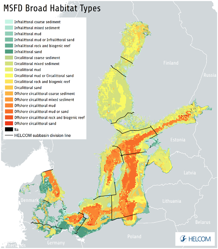
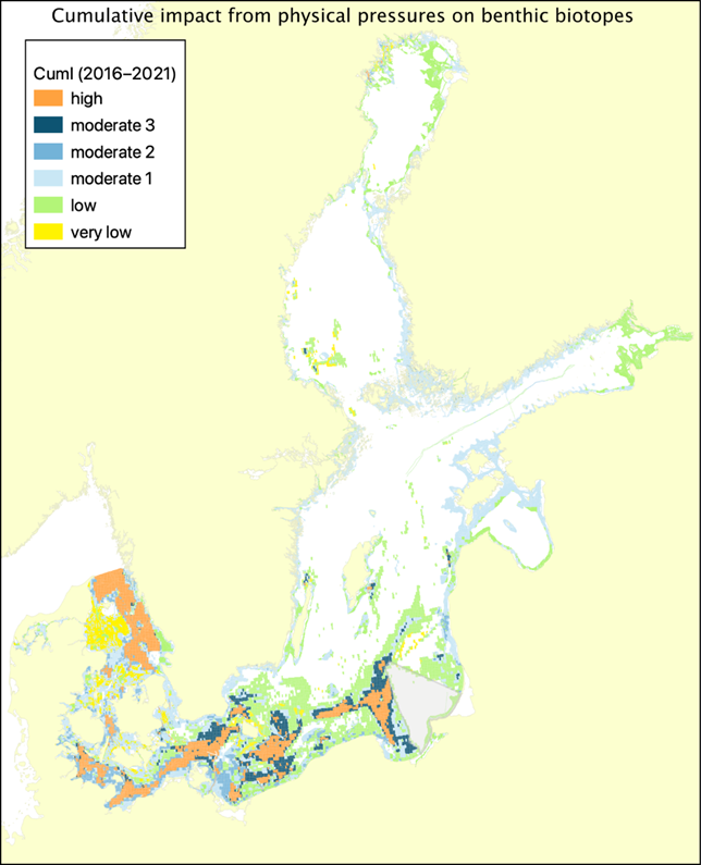
- Physical loss is defined at pressure level and its definition is part of the ongoing work in the EU technical group TG Seabed. Further development in the future is expected which will support greater harmonisation (e.g. on the definition and potential to consider other forms of loss/potential loss). ↑
- Unlike the dynamic sensitivity used in the OSPAR BH3 indicator. ↑
- https://helcom.fi/action-areas/monitoring-and-assessment/monitoring-manual/ ↑
- Note that the term ‘biotope’ here implies that the CumI does not evaluate the abiotic habitats as such (i.e. the BHTs) but assumes a living biocenosis in each BHT, leading to biotopes having specific sensitivities towards the various physical pressures. ↑