 Phytoplankton
2 Relevance of the indicator
Phytoplankton are the key primary producers in marine ecosystems. The phytoplankton community is comprised of several functionally diverse groups that dominate at different times of the year. Changes in the presence of specific phytoplankton group or the timing of when it dominates and becomes abundant may influence ecosystem function. The consequent altered timing of food and carbon availability for other higher trophic levels (e.g. zooplankton) can have wider food web impacts and the sedimentation of detritus (e.g. dead phytoplankton) can influence the microbial food web and ecosystem balance (e.g. heterotrophy-autotrophy) and the physicochemical state of the ecosystem (e.g. oxygen concentration).
A deviation from the normal seasonal cycle (such as a too high or too low biomass, or absence of some dominating phytoplankton group(s)) is indicative of an impairment of environmental status. Phytoplankton species composition changes if the amount of nutrients or the ratios of important nutrients (e.g. nitrogen and phosphorus) change, and eutrophication has resulted in more intense and frequent phytoplankton blooms during the summer.
2.1 Ecological relevance
Phytoplankton are the main primary producers in the marine pelagic ecosystem. These organisms occur in vast numbers and capture sunlight via photosynthesis to build biomass. These primary producers are commonly autotrophic and photosynthetic (though some can be mixotrophic) and they form a direct link between the environmental conditions (e.g. nutrient status) and the marine food webs. Phytoplankton biomass represents the base of the classical marine food web, forming the carbon and energy (and nutrient) source for grazers and predators such as zooplankton, which in turn are eaten by fish. Furthermore, phytoplankton can also play a role in the regulation of secondary basal producers (i.e. bacteria) that classically rely on exudates, and the degradation of phytoplankton biomass has consequences for biochemical cycles, such as oxygen consumption, and thus the status of the marine environment.
In aquatic ecosystems, a hierarchical response across trophic levels is commonly observed. Because of this, higher trophic levels may show a more delayed response or a weaker response to eutrophication than lower ones. Measurements of biomass (rather than abundance) were used to develop this indicator, since they can readily be translated into understanding biogeochemical cycles, they link to eutrophication, and are considered to give a more accurate depiction of the phytoplankton community. The succession of phytoplankton has a rather regular pattern and the initial event like spring bloom may also influence the formation of summer communities. Firstly, the dominance of either diatoms or dinoflagellates in the spring period determines the rate of sinking organic matter and subsequent oxygen consumption in bottom sediments. The diatoms settle out quickly and may cause oxygen depletion, which may in turn launch the release of phosphorus from sediments. This favours those phytoplankton which benefits from excessive phosphorus, especially bloom-forming diazotrophic (nitrogen fixing) cyanobacteria (e. g. Eilola et al., 2009).
The succession of dominant groups can provide an index that represents a healthy planktonic system, with a natural succession of dominant functional groups throughout the seasonal cycle. Deviations from the normal seasonal cycle, such as a too high or too low biomass, absence or appearance of some dominating groups at unusual time periods of the year, may indicate impairment in environmental status.
2.2 Policy relevance
Most pelagic habitats in the Baltic Sea are currently not in a healthy state and signs of deterioration at the food web and ecosystem levels are becoming more widespread and frequent. The pre-core indicator is among the few indicators able to evaluate the structure of the Baltic Sea food web, since phytoplankton have known links between environmental conditions (e.g. nutrient conditions) and higher trophic levels. Furthermore they have an important influence on other environmental or ecosystem components such as the supplementation of the microbial food web and possible consequences for oxygen conditions. Evaluations on the structure and functioning of the marine food web are requested by the Baltic Sea Action Plan (BSAP 2021) and the EU Marine Strategy Framework Directive (MSFD).
The EU MSFD lists a specific qualitative descriptor for the food webs: ‘All elements of the marine food webs, to the extent that they are known, occur at normal abundance and diversity and levels capable of ensuring the long-term abundance of the species and the retention of their full reproductive capacity.’
The pre-core indicator is also relevant in supporting a determination of good environmental status under MSFD Descriptor 1 Criteria 6 on pelagic habitats and Descriptor 5 Criteria 3 on harmful algae bloom (Commission Decision (EU) 2017/848).
Table 1. Policy relevance of the pre-core indicator
| Baltic Sea Action Plan (BSAP) | Marine Strategy Framework Directive (MSFD) | |
| Fundamental link | Segment: Biodiversity
Goal: “Baltic Sea ecosystem is healthy and resilient” Ecological objectives:
Management objective:
|
Descriptor 4 Ecosystems, including food webs
|
| Complementary link | Segment: Eutrophication
Goal: “Baltic Sea unaffected by eutrophication”
|
Descriptor 1 Species groups of birds, mammals, reptiles, fish and cephalopods
Descriptor 5 Ecosystems, including food webs
|
| Other relevant legislation: | UN Sustainable Development Goal 14 (Conserve and sustainably use the oceans, seas and marine resources for sustainable development) is most clearly relevant, though SDG 12 (Ensure sustainable consumption and production patterns) and 13 (Take urgent action to combat climate change and its impacts) also have relevance. | |
2.3 Relevance for other assessments
The status of biodiversity and food webs can be assessed using several core indicators. Each indicator focuses on one important aspect of the complex issue. In addition to providing an indicator-based evaluation of the “Seasonal succession of dominating phytoplankton groups”, this indicator will in the future also contribute to an overall food webs assessment, along with the other biodiversity core indicators. The seasonal succession indicator may also be used as background data for the development of a modified lifeform approach in the monitoring and environmental assessments in the HELCOM area. Lifeform approach has been considered to be taken into use in the MSFD assessments by OSPAR (Gowen et al. 2011, McQuatters-Gollop et al. 2019).
3 Threshold values
The concept for evaluating good environmental status using the succession of dominant groups in the phytoplankton community is structured around a reference status succession and the acceptable deviation from that pattern. The indicator evaluates the coincidence of seasonal succession of dominating phytoplankton groups over an assessment period (commonly 5−6 years) using regionally established reference seasonal growth curves and wet weight biomass data. The indicator result value is based on the number of data points falling within the acceptable deviation range set for each monthly point of the reference growth curve and expressed as the percentage to the total number of data points. This result value is then compared to regionally relevant threshold values established to represent acceptable levels of variation. Strong deviations from the reference growth curves will result in failure to meet the thresholds set for acceptable variation, indicating impairment of the environmental status and a failure to meet good status (Figure 2).
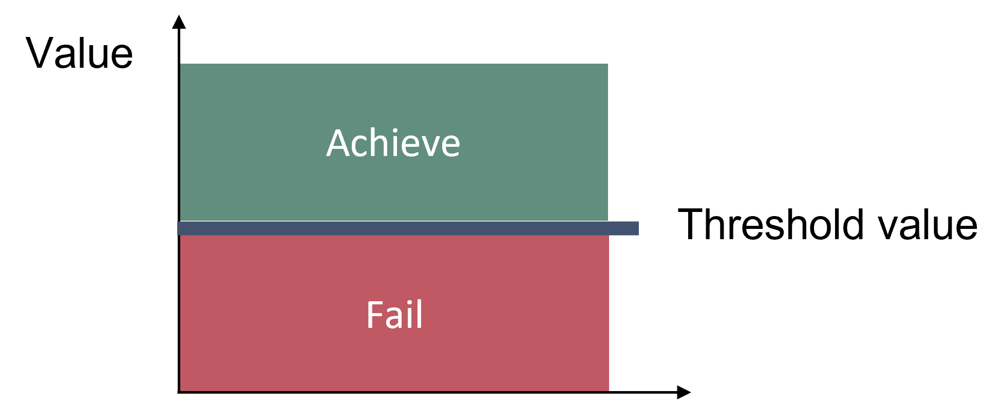
Figure 2. Good status is achieved when the indicator result (number of data points that fall within the established acceptable variation range) is above the regionally defined threshold value.
The specific regional threshold values used in this indicator are presented in Table 2. The final evaluation is based on the average score of single dominant groups. The threshold values are calculated for the periods with lower biomass values and lower interannual variability. If the number of deviations in an assessment unit increases along with the decreasing biomass values reflecting rather improvement in the ecological status, reference period may need to be redefined and threshold value recalculated. Therefore, part of the threshold values may be subjects of possible change for the next assessment period.
Table 2. Threshold values for selected assessment units in the Baltic Sea area, expressed as ratio of data points falling within the acceptable deviation range set for each monthly point.
| HELCOM Assessment unit ID and name | Threshold value |
| SEA-001 Kattegat | 0.56 |
| SEA-004 Kiel Bay | 0.55 |
| SEA-005 Bay of Mecklenburg | 0.61 |
| SEA-006 Arkona Basin | 0.55 |
| SEA-007 Bornholm Basin | 0.66 |
| SEA-008 Gdansk Basin | 0.61 |
| SEA-009 Eastern Gotland Basin | 0.68 |
| SEA-010 Western Gotland Basin | 0.70 |
| SEA-011 Gulf of Riga | 0.68 |
| SEA-012 Northern Baltic Proper | 0.70 |
| SEA-013 Gulf of Finland | 0.70 |
| SEA-015 Bothnian Sea | 0.63 |
| SEA-017 Bothnian Bay | 0.61 |
| 1 Bothnian Bay Finnish Coastal waters | 0.56 |
| 3 The Quark Finnish Coastal waters | 0.63 |
| 4 The Quark Swedish Coastal waters | 0.55 |
| 7 Åland Sea Finnish Coastal waters | 0.74 |
| 11 Gulf of Finland Finnish Coastal waters | 0.79 |
| 12 Gulf of Finland Estonian Coastal waters, western part | 0.65 |
| 12 Gulf of Finland Estonian Coastal waters, eastern part | 0.66 |
| 14 Gulf of Riga Estonian Coastal waters | 0.68 |
| 15 Gulf of Riga Latvian Coastal waters | 0.66 |
| 16 Western Gotland Basin Swedish Coastal waters | 0.71 |
| 19 Eastern Gotland Basin Lithuanian Coastal waters | 0.66 |
| 24 Gdansk Basin Polish Coastal waters | 0.60 |
| 32 Mecklenburg Bight German Coastal waters | 0.62 |
| 35 Kiel Bight German Coastal waters | 0.63 |
3.1 Setting the threshold value(s)
Background information on deriving the threshold values
The term ‘Good status’ has, however, to be taken with care as the first eutrophication affected changes in ecosystems emerged already in the mid-1950s in the Baltic Sea (Andersen et al., 2015). Only in a few basins, regular phytoplankton datasets date back to the mid-1980s (Table 3). Mostly the observations begin from the 1990s and in several coastal assessment units, regular sampling started only in 2006-2007 after the implementation of the Water Framework Directive. This means that most areas of the Baltic Sea have been heavily influenced by anthropogenic pressures prior to the initiation of regular monitoring and it may thus be difficult to determine reference conditions for the succession, based on pristine environmental conditions. Due to the lack of confirmed high status waterbodies or historical datasets, the reference seasonal growth curves have been set through observations made after the 1980s and the threshold between GES and sub-GES status is based on expert judgement.
To define unit-specific reference conditions, the periods of stability in long-term biomass data were ascertained. This approach was tested by calculating 5-year moving averages of standard deviations in yearly total biomass values (Figure 2). The recommended minimum time period for setting reference is ten years to include all natural variability. If it is not possible to determine a time period of sufficient length, the reference period can be split. As the data has been updated since the previous evaluation, also the reference periods and threshold values have been subjects of change. Further analysis with data seemed to indicate that in several cases, the deviations from the long-term mean reference growth curves have become less frequent during the last decade than in the 1990s and the early 2000s (Figure 4). This may infer an improvement in the current environmental status. For this reason, compared to the previous evaluation, reference periods and threshold values have changed in the Gulf of Gdansk and in the Gulf of Riga Latvian coastal waters. Minor changes have been made in most assessment units.
The threshold values based on calculations with data points representing reference periods varied from 0.55 (Arkona Basin and the Quark Swedish Coastal waters) to 0.79 (Gulf of Finland Finnish Coastal waters). Most of the threshold values fell within the range 0.6-0.7. This means that during the reference period, approximately 2/3 of observations fit within the acceptable deviation range from the reference growth curves.
Low threshold values should indicate high natural variability in seasonal succession of dominating phytoplankton groups and vice versa. In general, phytoplankton community structure and timely performance of dominant groups are more predictable in the areas with stable hydrological conditions (e.g. no major freshwater discharges and turbulent mixing). Offshore communities might have more coherent responses across the sea than coastal communities that tend to be more isolated and may therefore show little coherence within and among regions (Griffiths et al., 2015). This is also visible in the reference periods, which tend to be more similar in the adjacent open sea basins in comparison with the coastal assessment units belonging to the same sub-basin (Figure 4). Another reason explaining such discrepancy is due to different time periods of regular monitoring between the coastal and open sea areas.
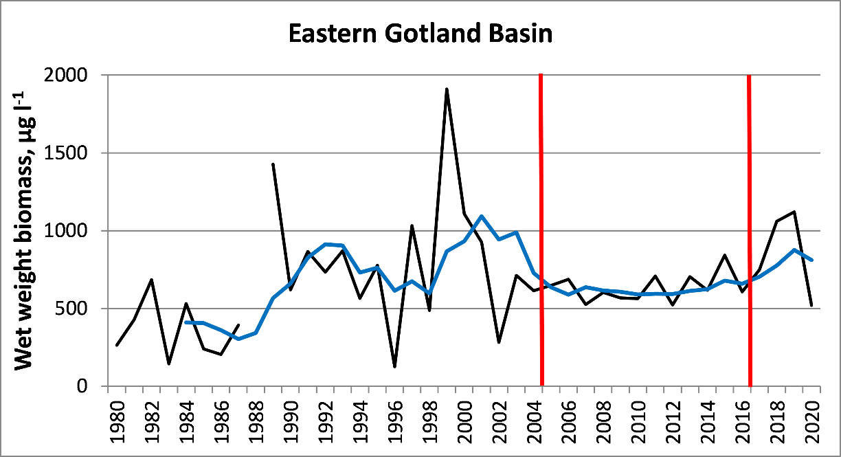
Figure 3. Selection of reference period by calculating 5-years moving averages (blue line) from yearly standard deviations of total phytoplankton biomass values (black line; µg l-1). The period with lowest variability is indicated between red bars.
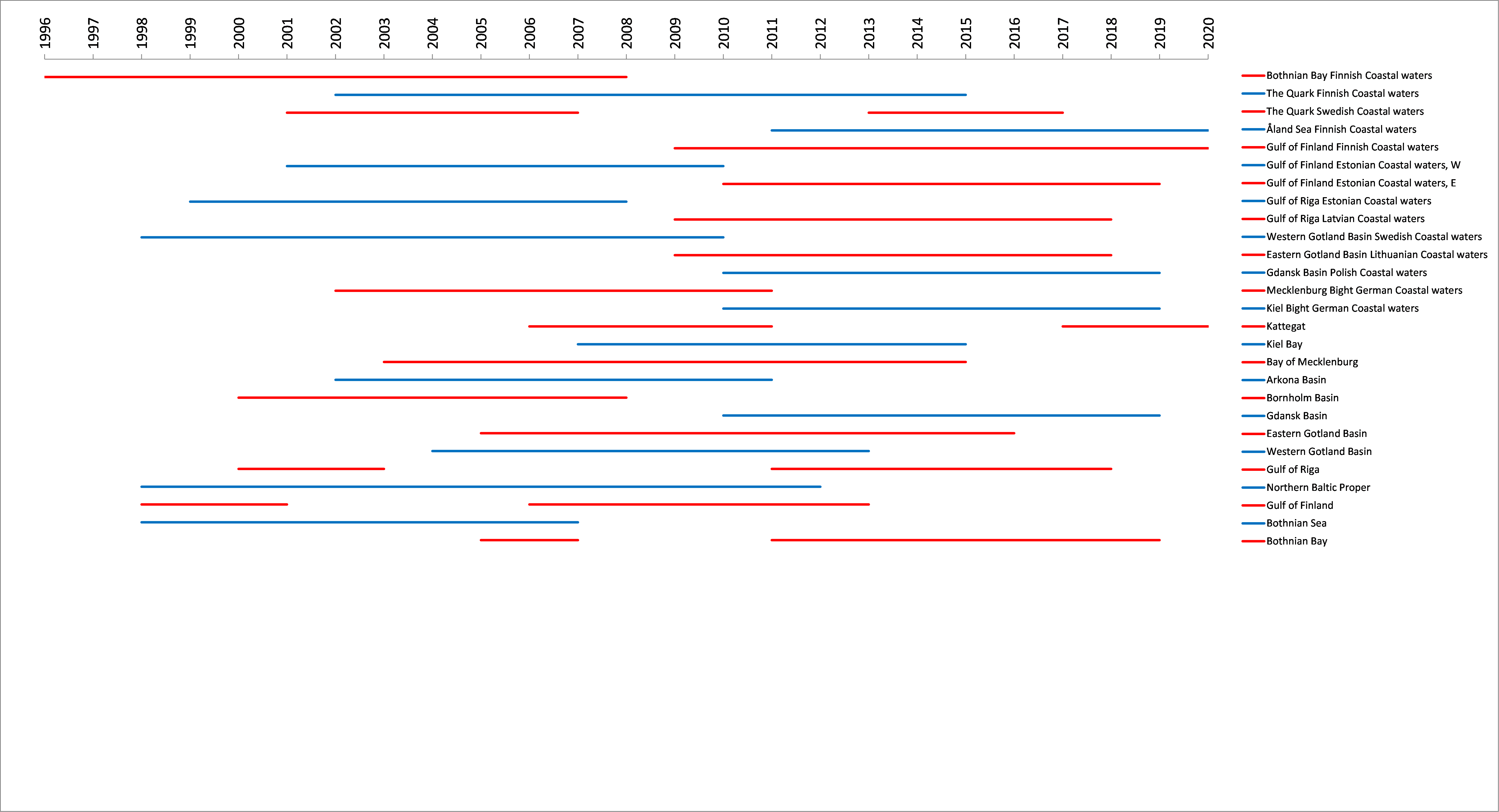
Figure 4. Scope of reference periods for seasonal succession of dominating phytoplankton groups in different assessment units across the Baltic Sea. Bars represent reference periods in the specific area, with alternating blue and red colours added to enhance readability.
4 Results and discussion
Below, the results of the indicator evaluation underlying the key message map and information are provided.
4.1 Status evaluation
The evaluation results are presented for 13 open sea basins out of 17 and for 13 coastal assessment units out of 40 (Table 3). In the Gulf of Finland Estonian coastal waters, western and eastern parts are evaluated separately due to salinity gradient and differences in phenology resulting in shifts of occurrence of dominant groups. The assessment units, excluded from the indicator analysis, are not monitored with sufficient frequency and regularity (incl. too short datasets to define reference period) or no data provided.
An example of reference growth curves and indicator values within the given assessment period is represented in Figure 5.
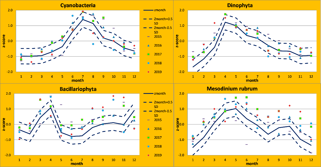
Figure 5. Reference growth curves with monthly averaged normalized biomass values (Zmonth), acceptable deviations (Zmonth±0.5) and data points during the period 2015-2019 in the Eastern Gotland Basin.
Table 3. Indicator results for the period 2015-2020 in comparison with threshold values in different assessment units of the Baltic Sea. The indicator value lies between 0 and 1 and is the proportion of data points within the “envelope” of seasonal reference growth curves and acceptable deviations. Data point is the average of all observations in a month of certain year. For overall evaluation, indicator values of individual dominant groups are averaged.
| HELCOM assessment unit name and ID | No. of stations | No. of obs./ data points (2015-2020) | Dominant groups | Indicator value | Threshold value | Reference period | Beginning of regular monitoring |
| SEA-001 Kattegat | 2 | 174/66 | All groups
Cyanobacteria Dinoflagellates Diatoms M. rubrum |
0.55
0.71 0.62 0.35 0.50 |
0.56
0.75 0.58 0.38 0.54 |
2006–2011;
2017–2020 |
1994 |
| SEA-004 Kiel Bay | 2 | 150/61 | All groups
Cyanobacteria Dinoflagellates Diatoms M. rubrum |
0.50
0.75 0.49 0.31 0.46 |
0.55
0.76 0.56 0.44 0.43 |
2007–2015 | 2007 |
| SEA-005 Bay of Mecklenburg | 2 | 148/59 | All groups
Cyanobacteria Dinoflagellates Diatoms M. rubrum |
0.60
0.71 0.56 0.46 0.68 |
0.61
0.80 0.57 0.47 0.61 |
2003–2015 | 1980 |
| SEA-006 Arkona Basin | 6 | 172/57 | All groups
Cyanobacteria Dinoflagellates Diatoms M. rubrum |
0.61
0.63 0.58 0.56 0.67 |
0.55
0.54 0.58 0.53 0.56 |
2002–2011 | 1980 |
| SEA-007 Bornholm Basin | 4 | 148/54 | All groups
Cyanobacteria Dinoflagellates Diatoms M. rubrum |
0.54
0.57 0.61 0.43 0.56 |
0.66
0.68 0.67 0.61 0.68 |
2000–2008 | 1980 |
| SEA-008 Gdansk Basin | 3 | 28/20 | All groups
Cyanobacteria Dinoflagellates Diatoms M. rubrum |
0.67
0.71 0.71 0.75 0.50 |
0.61
0.65 0.65 0.65 0.47 |
2010–2019 | 1984 |
| SEA-009 Eastern Gotland Basin | 5 | 170/64 | All groups
Cyanobacteria Dinoflagellates Diatoms M. rubrum |
0.64
0.71 0.75 0.56 0.70 |
0.68
0.67 0.63 0.53 0.73 |
2005–2016 | 1980 |
| SEA-010 Western Gotland Basin | 2 | 114/58 | All groups
Cyanobacteria Dinoflagellates Diatoms M. rubrum |
0.56
0.71 0.64 0.50 0.38 |
0.70
0.76 0.74 0.62 0.66 |
2004–2013 | 1990 |
| SEA-011 Gulf of Riga | 13 | 197/44 | All groups
Cyanobacteria Dinoflagellates Diatoms M. rubrum |
0.51
0.36 0.57 0.57 0.52 |
0.68
0.61 0.79 0.65 0.66 |
2000–2003; 2011-2018 | 1992 |
| SEA-012 Northern Baltic Proper | 3 | 184/64 | All groups
Cyanobacteria Dinoflagellates Diatoms M. rubrum |
0.57
0.73 0.66 0.52 0.39 |
0.70
0.73 0.74 0.60 0.72 |
1998–2012 | 1990 |
| SEA-013 Gulf of Finland | 4 | 108/32 | All groups
Cyanobacteria Dinoflagellates Diatoms M. rubrum |
0.62
0.66 0.69 0.69 0.44 |
0.70
0.84 0.68 0.78 0.48 |
1997-2012 | 1990 |
| SEA-015 Bothnian Sea | 4 | 56/46 | All groups
Cyanobacteria Dinoflagellates Diatoms M. rubrum |
0.45
0.57 0.49 0.31 0.43 |
0.63
0.61 0.67 0.61 0.64 |
1993-2004 | 1995 |
| SEA-017 Bothnian Bay | 5 | 55/47 | All groups
Cyanobacteria Dinoflagellates Diatoms M. rubrum |
0.65
0.68 0.77 0.55 0.62 |
0.61
0.59 0.75 0.53 0.59 |
2001-2015 | 1995 |
| 1 Bothnian Bay Finnish Coastal waters | 28 | 282/36 | All groups
Cyanobacteria Dinoflagellates Diatoms M. rubrum |
0.47
0.42 0.58 0.47 0.42 |
0.56
0.33 0.82 0.60 0.47 |
1996–2008 | 1990 |
| 3 The Quark Finnish Coastal waters | 8 | 142/37 | All groups
Cyanobacteria Dinoflagellates Diatoms M. rubrum |
0.43
0.59 0.19 0.51 0.43 |
0.63
0.70 0.55 0.61 0.68 |
2002–2015 | 1998 |
| 4 The Quark Swedish Coastal waters | 2 | 49/45 | All groups
Cyanobacteria Dinoflagellates Diatoms M. rubrum |
0.71
0.64 0.73 0.69 0.64 |
0.55
0.56 0.57 0.52 0.58 |
2001–2007; 2013–2017 | 1995 |
| 7 Åland Sea Finnish Coastal waters | 51 | 677/32 | All groups
Cyanobacteria Dinoflagellates Diatoms M. rubrum |
0.71
0.75 0.53 0.88 0.69 |
0.74
0.85 0.63 0.74 0.73 |
2011–2020 | 1990 |
| 11 Gulf of Finland Finnish Coastal waters | 37 | 782/48 | All groups
Cyanobacteria Dinoflagellates Diatoms M. rubrum |
0.78
0.69 0.71 0.90 0.83 |
0.79
0.67 0.79 0.84 0.85 |
2009–2020 | 1990 |
| 12 Gulf of Finland Estonian Coastal waters, western part | 3 | 195/42 | All groups
Cyanobacteria Dinoflagellates Diatoms M. rubrum |
0.49
0.52 0.60 0.43 0.43 |
0.65
0.73 0.64 0.75 0.47 |
2001–2010 | 1993 |
| 12 Gulf of Finland Estonian Coastal waters, eastern part | 3 | 190/42 | All groups
Cyanobacteria Dinoflagellates Diatoms M. rubrum |
0.63
0.55 0.57 0.74 0.64 |
0.66
0.63 0.60 0.75 0.69 |
2010–2019 | 1990 |
| 14 Gulf of Riga Estonian Coastal waters | 3 | 213/41 | All groups
Cyanobacteria Dinoflagellates Diatoms M. rubrum |
0.61
0.54 0.68 0.73 0.49 |
0.68
0.63 0.80 0.68 0.62 |
1999–2008 | 1993 |
| 15 Gulf of Riga Latvian Coastal waters | 11 | 236/41 | All groups
Cyanobacteria Dinoflagellates Diatoms M. rubrum |
0.68
0.66 0.71 0.68 0.66 |
0.66
0.56 0.76 0.73 0.60 |
2009–2018 | 1995 |
| 16 Western Gotland Basin Swedish Coastal waters | 2 | 201/72 | All groups
Cyanobacteria Dinoflagellates Diatoms M. rubrum |
0.64
0.79 0.76 0.40 0.58 |
0.71
0.79 0.74 0.68 0.63 |
1998–2010 | 1983 |
| 19 Eastern Gotland Basin Lithuanian Coastal waters | 7 | 165/45 | All groups
Cyanobacteria Dinoflagellates Diatoms M. rubrum |
0.62
0.67 0.69 0.51 0.62 |
0.66
0.72 0.69 0.48 0.62 |
2009–2018 | 2001 |
| 24 Gdansk Basin Polish Coastal waters | 22 | 65/44 | All groups
Cyanobacteria Dinoflagellates Diatoms M. rubrum |
0.56
0.55 0.59 0.59 0.52 |
0.60
0.57 0.59 0.59 0.64 |
2010–2019 | 1987 |
| 32 Mecklenburg Bight German Coastal waters | 6 | 238/53 | All groups
Cyanobacteria Dinoflagellates Diatoms M. rubrum |
0.64
0.72 0.68 0.49 0.66 |
0.62
0.57 0.75 0.56 0.59 |
2002–2011 | 1997 |
| 35 Kiel Bight German Coastal waters | 5 | 169/48 | All groups
Cyanobacteria Dinoflagellates Diatoms M. rubrum |
0.65
0.76 0.60 0.51 0.57 |
0.63
0.74 0.65 0.52 0.59 |
2010–2019 | 2007 |
Please note that German coastal waters were not part of this evaluation but that WFD results were used instead and are thus displayed accordingly in Figure 1, where a good WFD status is displayed as achieved and anything else as failed. The results in table 4 show the WFD results for German coastal waters.
Table 4. Results for German coastal waters are from the WFD and result based on the biological quality component phytoplankton.
| Unit ID | Unit Code | Unit Description | Chl-a [µg/l] | Assessment class Chl-a | Phytoplankton Index [EQR] | Assessment class Phytoplankton Index |
| 1001 | GER-001 | mesohaline inner coastal waters, Wismarbucht, Suedteil | 0.5718 | moderate | ||
| 1002 | GER-002 | mesohaline inner coastal waters, Wismarbucht, Nordteil | 0.5718 | moderate | ||
| 1003 | GER-003 | mesohaline inner coastal waters, Wismarbucht, Salzhaff | 0.5210 | moderate | ||
| 1004 | GER-004 | mesohaline open coastal waters, Suedliche Mecklenburger Bucht/ Travemuende bis Warnemünde | 0.4968 | moderate | ||
| 1005 | GER-005 | mesohaline inner coastal waters, Unterwarnow | 0.5214 | moderate | ||
| 1006 | GER-006 | mesohaline open coastal waters, Suedliche Mecklenburger Bucht/ Warnemünde bis Darss | 0.4261 | moderate | ||
| 1007 | GER-007 | oligohaline inner coastal waters, Ribnitzer See / Saaler Bodden | 0.1760 | bad | ||
| 1008 | GER-008 | oligohaline inner coastal waters, Koppelstrom / Bodstedter Bodden | 0.2597 | poor | ||
| 1009 | GER-009 | mesohaline inner coastal waters, Barther Bodden, Grabow | 0.1837 | bad | ||
| 1010 | GER-010 | mesohaline open coastal waters, Prerowbucht/ Darsser Ort bis Dornbusch | 0.8720 | good | ||
| 1011 | GER-011 | mesohaline inner coastal waters, Westruegensche Bodden | 0.3780 | poor | ||
| 1012 | GER-012 | mesohaline inner coastal waters, Strelasund | 0.3677 | poor | ||
| 1013 | GER-013 | mesohaline inner coastal waters, Greifswalder Bodden | 0.3820 | poor | ||
| 1014 | GER-014 | mesohaline inner coastal waters, Kleiner Jasmunder Bodden | 0.1800 | bad | ||
| 1015 | GER-015 | mesohaline open coastal waters, Nord- und Ostruegensche Gewaesser | 0.5119 | moderate | ||
| 1016 | GER-016 | oligohaline inner coastal waters, Peenestrom | 0.2722 | poor | ||
| 1017 | GER-017 | oligohaline inner coastal waters, Achterwasser | 0.2364 | poor | ||
| 1018 | GER-018 | mesohaline open coastal waters, Pommersche Bucht, Nordteil | 0.3493 | poor | ||
| 1019 | GER-019 | mesohaline open coastal waters, Pommersche Bucht, Südteil | 0.2779 | poor | ||
| 1020 | GER-020 | oligohaline inner coastal waters, Kleines Haff | 0.2821 | poor | ||
| 1021 | GER-021 | mesohaline inner coastal waters, Flensburg Innenfoerde | 5.0850 | poor | ||
| 1022 | GER-022 | mesohaline open coastal waters, Geltinger Bucht | 2.0418 | moderate | ||
| 1023 | GER-023 | meso- to polyhaline open coastal waters, seasonally stratified, Flensburger Aussenfoerde | 2.0418 | moderate | ||
| 1024 | GER-024 | mesohaline open coastal waters, Aussenschlei | 2.0553 | moderate | ||
| 1025 | GER-025 | mesohaline inner coastal waters, Schleimuende | 21.6758 | bad | ||
| 1026 | GER-026A | A.mesohaline inner coastal waters, Mittlere Schlei | 53.3100 | bad | ||
| 1027 | GER-026B | B.mesohaline inner coastal waters, Mittlere Schlei | 68.3740 | bad | ||
| 1028 | GER-027 | mesohaline inner coastal waters, Innere Schlei | 68.3740 | bad | ||
| 1029 | GER-028 | mesohaline open coastal waters, Eckerfoerder Bucht, Rand | 1.7330 | good | ||
| 1030 | GER-029 | meso- to polyhaline open coastal waters, seasonally stratified, Eckerfoerderbucht, Tiefe | 1.9657 | moderate | ||
| 1031 | GER-030 | mesohaline open coastal waters, Buelk | 1.9657 | moderate | ||
| 1032 | GER-031 | meso- to polyhaline open coastal waters, seasonally stratified, Kieler Aussenfoerde | 2.0357 | moderate | ||
| 1033 | GER-032 | mesohaline inner coastal waters, Kieler Innenfoerde | 4.5272 | poor | ||
| 1034 | GER-033 | mesohaline open coastal waters, Probstei | 1.8000 | good | ||
| 1035 | GER-034 | mesohaline open coastal waters, Putlos | 1.8000 | good | ||
| 1036 | GER-035 | meso- to polyhaline open coastal waters, seasonally stratified, Hohwachter Bucht | 1.6492 | good | ||
| 1037 | GER-036A | A.mesohaline open coastal waters, Fehmarnsund | 1.7680 | good | ||
| 1038 | GER-036B | B.mesohaline open coastal waters, Fehmarnsund | 1.7860 | good | ||
| 1039 | GER-037 | mesohaline inner coastal waters, Orther Bucht | 1.8623 | good | ||
| 1040 | GER-038A | A.mesohaline open coastal waters, Fehmarnbelt | 1.4699 | good | ||
| 1041 | GER-038B | B.mesohaline open coastal waters, Fehmarnbelt | 1.4699 | good | ||
| 1042 | GER-039 | meso- to polyhaline open coastal waters, seasonally stratified, Fehmarn Sund Ost | 1.5851 | good | ||
| 1043 | GER-040 | mesohaline open coastal waters, Groemitz | 2.1330 | moderate | ||
| 1044 | GER-041 | mesohaline open coastal waters, Neustaedter Bucht | 2.1957 | moderate | ||
| 1045 | GER-042 | mesohaline inner coastal waters, Travemuende | 19.7657 | bad | ||
| 1046 | GER-043 | mesohaline inner coastal waters, Poetenitzer Wiek | 19.7657 | bad | ||
| 1047 | GER-044 | mesohaline inner coastal waters, Untere Trave | 20.1872 | bad | ||
| 1048 | GER-111 | mesohaline inner coastal waters, Nordruegensche Bodden | 0.2250 | poor |
4.2 Trends
Distinct trends between the current and previous evaluation are considered if there is a difference in the indicator values equal or more than 15% (HELCOM, 2018). Indicator values for the previous period (2011–2016) have been also calculated in the assessment units not included in HOLAS II. The changes in groups do not follow the same trends in all areas and an increase or a decrease in the same group in different areas can only be evaluated against the specific reference period (threshold value setting period) for the region. The threshold value reflects the balance between the dominating groups from that period and the evaluation is carried out in relation to that. Thus, an increase or decrease in a group may alter the balance from the selected reference period, but changes alone in those groups are not themselves indicative of a specific directional change that can be used to infer status overall and must be considered as a change related to the balance between the groups relative to the threshold value setting period.
An overview is provided in Table 5.
Table 5. Assessment units, threshold values and trends
| HELCOM Assessment unit ID and name | Threshold value achieved/failed – HOLAS II | Threshold value achieved/failed – HOLAS 3 | Distinct trend between current and previous evaluation | Description of outcomes |
| SEA-001 Kattegat | Not evaluated | failed | NA | Increasing dinoflagellate and decreasing diatom biomass |
| SEA-004 Kiel Bay | Not evaluated | failed | NA | Increasing diatom and de-creasing dinoflagellate biomass |
| SEA-005 Bay of Mecklenburg | Not evaluated | failed | NA | Increasing cyanobacteria and diatom biomass |
| SEA-006 Arkona Basin | failed | achieved | Deterioration. The status has deteriorated in the current assessment period, possibly the availability of a larger data set compared to the test evaluation in the previous period plays a role in this change. | |
| SEA-007 Bornholm Basin | failed | failed | No change in status between assessment periods. | Increasing diatom and Mesodinium rubrum biomass |
| SEA-008 Gdansk Basin | achieved | achieved | No change in status between assessment periods. | |
| SEA-009 Eastern Gotland Basin | failed | failed | No change in status between assessment periods. | Decreasing dinoflagellate biomass |
| SEA-010 Western Gotland Basin | Not evaluated | failed | NA | Increasing diatom and Mesodinium rubrum biomass |
| SEA-011 Gulf of Riga | failed | failed | No change in status between assessment periods. | |
| SEA-012 Northern Baltic Proper | failed | failed | No change in status between assessment periods. | Increasing diatom and Mesodinium rubrum biomass |
| SEA-013 Gulf of Finland | Not evaluated | failed | NA | Increasing diatom and Mesodinium rubrum biomass |
| SEA-015 Bothnian Sea | Not evaluated | failed | NA | Increasing biomass in all dominant groups |
| SEA-017 Bothnian Bay | Not evaluated | achieved | NA | |
| 1 Bothnian Bay Finnish Coastal waters | failed | NA | Increasing biomass in all dominant groups, except dinoflagellates | |
| 3 The Quark Finnish Coastal waters | Not evaluated | failed | NA | Decreasing dinoflagellate and increasing Mesodinium rubrum biomass |
| 4 The Quark Swedish Coastal waters | Not evaluated | achieved | NA | |
| 7 Åland Sea Finnish Coastal waters | Not evaluated | failed | NA | |
| 11 Gulf of Finland Finnish Coastal waters | Not evaluated | failed | NA | |
| 12 Gulf of Finland Estonian Coastal waters, western part | failed | failed | No change in status between assessment periods. | Increasing diatom and Mesodinium rubrum biomass |
| 12 Gulf of Finland Estonian Coastal waters, eastern part | failed | failed | No change in status between assessment periods. | Increasing Mesodinium rubrum biomass |
| 14 Gulf of Riga Estonian Coastal waters | failed | failed | No change in status between assessment periods. | |
| 15 Gulf of Riga Latvian Coastal waters | failed | achieved | Positive. The status is approved in the current assessment period. | |
| 16 Western Gotland Basin Swedish Coastal waters | Not evaluated | failed | NA | Increasing diatom and Mesodinium rubrum biomass |
| 19 Eastern Gotland Basin Lithuanian Coastal waters | achieved | failed | No | Decreasing cyanobacterial biomass |
| 24 Gdansk Basin Polish Coastal waters | Not evaluated | failed | NA | Increasing Mesodinium rubrum biomass |
| 32 Mecklenburg Bight German Coastal waters | Not evaluated | achieved | NA | Increasing diatom biomass |
| 35 Kiel Bight German Coastal waters | Not evaluated | achieved | NA | Increasing cyanobacteria and diatom biomass |
4.3 Discussion text
Phytoplankton communities are comprised of several functionally diverse groups that dominate at different times of the year. The consequent altered timing of food and carbon availability for other higher trophic levels (e.g. zooplankton) can have wider food web impacts and the sedimentation of detritus (e.g. dead phytoplankton) can influence the microbial food web and ecosystem balance (e.g. heterotrophy-autotrophy) and the physicochemical state of the ecosystem (e.g. oxygen concentration). Phytoplankton species composition also changes if the amount of nutrients or the ratios of important nutrients (nitrogen and phosphorus) change, and eutrophication has resulted in more intense and frequent phytoplankton blooms.
The selected dominant groups for the seasonal succession indicator – cyanobacteria, dinoflagellates, diatoms and the autotrophic ciliate Mesodinium rubrum contribute usually at least 80–90% to the total phytoplankton biomass and make the base of marine food web. The relevance of different dominant groups is, however, highly variable across the Baltic Sea and mainly governed by salinity (e.g. Gasiūnaitė et al., 2005). It is most prominent in cyanobacteria, which make up 10-25% of the annual phytoplankton biomass in the northern (except Bothnian Bay), eastern and central parts of the Baltic Sea, but only 0.3-2% in the southern basins and the Kattegat. 21 assessment units out of 27 analysed for this indicator are more or less diatom dominated. However, a distinction must be made here, as in the northern and central parts of the Baltic Sea diatoms make the bulk biomass in spring period, while in the south and the Kattegat, the peak biomasses are observed rather in autumn. The contribution of diatoms to the annual biomass is the largest in the coastal waters of Bothnian Bay and in the Kattegat (85-86% among the four dominant groups) and only the three basins (northern Baltic Proper, eastern and western Gotland basins) are dinoflagellate dominated during the spring bloom. The autotrophic ciliate Mesodinium rubrum plays an important role in Bothnian Bay, Bothnian Sea, the Gulf of Riga and eastern and western Gotland basins (20–30% of annual biomass on average).
The results presented in 4.2 indicate that in comparison of previous and current assessment periods, most of the increasing trends in the biomasses of dominant groups are due to diatoms – in Bothnian Bay, Bothnian Sea, the Gulf of Finland, Northern Baltic Proper, Western Gotland Basin, Bay of Mecklenburg and Kiel Bay. The share of dinoflagellates has been increasing only in the Kattegat and Bothnian Sea between these two periods. Except the Bay of Mecklenburg and Kiel Bay, these changes concern the spring bloom, the period with the highest annual primary production and sinking of organic matter to the sediment. The fate of this organic matter is a key driver for material fluxes, affecting ecosystem functioning and eutrophication feedback loops. The dominant diatoms and dinoflagellates appear to be functionally surrogates as both groups are able to effectively exhaust the wintertime accumulation of inorganic nutrients and produce bloom level biomass that contribute to vertical export of organic matter (Kremp et al., 2008; Spilling et al., 2018). However, the groups have very different sedimentation patterns, and the seafloor has variable potential to mineralize the settled biomass in the different sub-basins. While diatoms sink quickly out of the euphotic zone, dinoflagellates sink as inert resting cysts, or decompose in the water column contributing to slowly settling phyto-detritus. The dominance by both phytoplankton group thus directly affects both the summertime nutrient pools of the water column and the input of organic matter to the sediment but to contrasting directions. The proliferation of dinoflagellates with high encystment efficiency could increase sediment retention and burial of organic matter, alleviating the eutrophication problem and improve the environmental status of the Baltic Sea. Thus, the increasing dominance of diatoms impacts sedimentation of phytoplankton biomass quantitatively, with higher vertical export of fixed carbon from the atmosphere to great depths (Smetacek, 1998). The conclusions must be drawn, however, with caution as we compare rather short time periods. Over a wider period before the 2010s, the proportion of dinoflagellates has been on the rise at least in the northernmost basins, in the gulfs of Bothnia and Finland (Klais et al., 2011).
In the northern and central basins, also the autotrophic ciliate M. rubrum indicates an upward trend between the two assessment periods. Intensive studies in the Gulf of Finland have revealed that the blooms of this species are more prominent in years of earlier warming in spring (Lips & Lips, 2017). An increase in cyanobacterial biomass was observed in the areas where blooms have not been common – Bothnian Bay, Bothnian Sea, Bay of Mecklenburg and Kiel Bight. Statistically significant increasing trend in the Bay of Mecklenburg and Western Gotland Basin has been also detected by Kownacka et al. (2021). The same authors have revealed decreasing trend in cyanobacterial biomass in the central parts of the Baltic Sea – Arkona, Bornholm and Eastern Gotland basins during 1990-2020.
At the same time, the overall evaluation results of the seasonal succession indicator show opposite trends in different sub-basins of the Baltic Sea. In the open sea assessment units, phytoplankton communities seem to be heading for greater stability in the southern parts (Arkona, Bornholm and Gdansk basins, the Bay of Mecklenburg), while in the northern assessment units and in the Western Gotland Basin the status is moving further from good.
It has been noted for this indicator, that it is challenging to define a threshold value for good or not good environmental status, and since defining status is a complex process when addressing complex systems such as food webs, an expression or understanding of change (or no change) may be a more appropriate way to evaluate food webs. This applies in particular where data may simply not be available from a non-disturbed period, e.g. without eutrophication effects. The indicator seasonal succession of dominating phytoplankton groups is therefore primarily not a status indicator, but rather reflects trends by comparison of reference and assessment periods. There is also a danger that increasing deviations judged as bad are in fact positive because they are caused by declining eutrophication. Furthermore, using a recent reference period means that we also include the impact of climate change which might be more influential than eutrophication.
5 Confidence
Confidence is assessed based on expert evaluation of the information that underlies the confidence scoring. Specifically, this requires a categorical scoring of four different criteria: accuracy of estimate (where if present standard error or statistical outputs are used), temporal coverage, spatial representability of data, and methodological confidence. Confidence can be scored as high, intermediate or low for these criteria. Temporal coverage is scored based on monitoring data cover during the assessment period (year range for assessment and variation such as temporal frequency). For spatial representability, spatial cover (e.g. patchiness) is evaluated. For methodological confidence, scoring of conducted monitoring and data quality are scored. The result for confidence in this phytoplankton pre-core indicator evaluation reflects all of these criteria. The approach is applied in all biodiversity indicators following harmonised guidance provide for the integrated biodiversity assessment tool (BEAT) so that these values can be utilised in downstream assessments. Spatio-temporal coverage differs between the assessment units. For most of the assessed areas, the confidence of indicator status is intermediate to high according to temporal and intermediate according to spatial resolution. Confidence level depends on the length of the time-series and regularity of phytoplankton sampling during the growth period. On the other hand, once the reference growth curves have been established, some compromises in the frequency of sampling and total number of samples used in the evaluation are possible. The indicator value is the proportion of biomass values fitting into the reference growth envelope (region of acceptable deviation) and the values for individual months are independent. It means that if some data points for some months are missing during the assessment period, the evaluation is still feasible.
Methodological confidence of monitoring data used for this indicator is rather high since all laboratories providing data follow the same guidelines. The quality of data is substantially improved after implementing a standardised species list with fixed size-classes and biovolumes (Olenina et al., 2006).
6 Drivers, Activities, and Pressures
The shift in the plankton community is most probably due to complex interactions between climate change impacts, eutrophication and increased top-down pressures due to overexploitation of resources, and the resulting trophic cascades. Eutrophication is commonly noted as being the major driver behind current impacts on the phytoplankton community. A shift in functional groups may affect ecosystem function in terms of the carbon available to higher trophic levels or settling to the sediments. The examination of seasonality shows the broad temporal variability of phytoplankton populations. Succession of dominant groups can potentially provide an index that represents a healthy planktonic system, with a natural progression of dominant functional groups throughout the seasonal cycle. Alterations in the seasonal cycle may be related to nutrient enrichment. Expert judgement must be used when alterations in the seasonal cycle, and their causes, are interpreted.
It has been pointed out that phytoplankton indicators show complex pressure-response relationships, and their use is therefore demanding. However, phytoplankton indicators have additional value for the implementation of the MSFD. Ecosystem components often respond non-linearly to environmental drivers and human stressors, where small changes in a driver cause a disproportionately large ecological response. In pelagic ecosystems, non-linearities comprise more than half of all driver-response relationships (Hunsicker et al., 2016). The effects of eutrophication on phytoplankton may be expressed by shifts in species composition and increases in the frequency and intensity of nuisance blooms.
Table 6. Brief summary of relevant pressures and activities with relevance to the indicator.
| | General | MSFD Annex III, Table 2a |
| Strong link | the most important anthropogenic threat to phytoplankton is eutrophication | Input of nutrients — diffuse sources, point sources, atmospheric deposition.
Input of organic matter — diffuse sources and point sources. |
| Weak link | Biological disturbance (introduction of non-native species) |
7 Climate change and other factors
Seasonal succession indicator also reflects climate-induced changes in phenology with the consequences on productivity and food webs. Phytoplankton phenology has even been proposed as an indicator to monitor systematically the state of the pelagic ecosystem and to detect changes triggered by perturbation of the environmental conditions (Racault et al., 2012). The duration of sunshine and sea surface temperature (SST) are the main factors governing the onset and the length of vegetation. At high-latitudes, higher SST is associated with prolongation of the growing period – both the earlier onset of spring bloom and the extension of phytoplankton peak biomasses during summer and autumn (Kahru et al., 2016; Racault et al., 2012; Sommer & Lewandowska, 2011; Wasmund et al., 2019). On the example of cyanobacteria, dominating mainly in the summer period, significantly higher growth rates and peak abundances have been measured in the average and warm spring scenarios than in the cold spring scenario (De Senerpont Domis et al., 2007).
Temperature has both a nutrient-independent effect and a nutrient-shared effect on phytoplankton community size structure (Askov Mousing et al., 2014). Although the correlation between the duration of the growing season and the concentrations of nutrients may not be causative, the macroecological patterns show an increase in the fraction of large phytoplankton with increasing nutrient availability and a decrease with increasing temperature. Response of phytoplankton to precipitation depends upon the season and region. Using long-term time-series data worldwide, Thompson et al. (2015) concluded that in general phytoplankton responded more positively to increased precipitation during summer rather than winter. Analyses in Chesapeake Bay revealed increased abundance of diatoms in wet years compared to long-term average or dry years (Harding et al., 2015).
It is predictable that the community structure becomes increasingly unstable in response to climate change (Henson et al., 2021). Here is also a direct reference to the seasonal succession indicator, where the deviations from the reference growth patterns reflect impairment in the environmental status.
8 Conclusions
The indicator evaluates the coincidence of seasonal succession of dominating phytoplankton groups over an assessment period (commonly 5−6 years) with regionally established reference seasonal growth curves using wet weight biomass data. Deviations from the normal seasonal cycle may indicate impairment in the environmental status.
Phytoplankton data are not available from a non-disturbed period, e.g. without eutrophication effects. Status may be highly complex to define and an expression or understanding of change (or no change) may be a more appropriate way for the evaluation. The seasonal succession of dominating phytoplankton groups is therefore primarily not a status indicator, but rather reflects trends by comparison of reference and assessment periods.
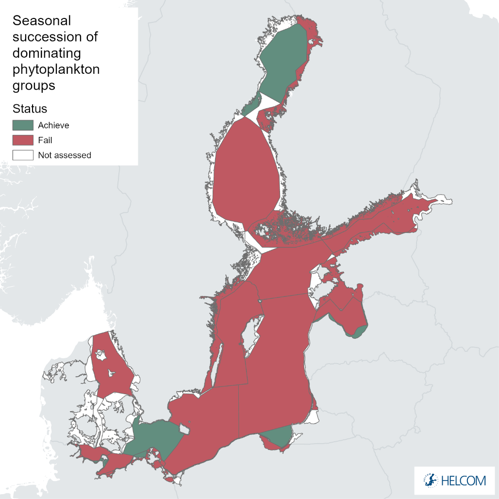
The status evaluation has been done for specific assessment units over the period 2015–2020. The assessment results are presented for 13 open sea basins out of 17 and for 13 coastal assessment units out of 40. GES has been achieved in two open sea basins and in four coastal water assessment units.
Most of the increasing trends in the biomasses of dominant groups are due to diatoms. The dominance of either diatoms or dinoflagellates in the spring period determines the rate of sinking organic matter and subsequent oxygen consumption in bottom sediments. The diatoms settle out quickly and may cause oxygen depletion, which may in turn launch the release of phosphorus from sediments. This can favour blooms of diazotrophic (nitrogen fixing) cyanobacteria, which benefits from excessive phosphorus.
An upward biomass trend of the autotrophic ciliate Mesodinium rubrum in the northern and central basins of the Baltic Sea may be related to earlier warming in spring.
In the southern Baltic Sea (Arkona, Bornholm and Gdansk basins, the Bay of Mecklenburg), phytoplankton communities seem to be heading for greater stability, while in the northern assessment units and in the Western Gotland Basin the deviations from the normal succession growth curves have become more frequent.
The confidence of indicator status is intermediate to high according to temporal and intermediate according to spatial resolution. Methodological confidence of monitoring data used for this indicator is rather high since all laboratories providing data follow the same guidelines.
8.1 Future work or improvements needed
In some areas, especially offshore, phytoplankton monitoring can be supported by FerryBox sampling. For time being, microscopic analysis is a part of Ferrybox sampling only in the Estonian and Swedish monitoring programs.
Additional work could be explored in relation to linking the threshold values (and periods applied) to a harmonised period known to reflect an environmental condition that is classified as good (e.g. a pre-eutrophication impacted state). Another issue that could be further explored is the handling of imbalances and gaps in data sets. Future work on this indicator could further aim on strengthening the rationale for the indicator, including demonstrating the link to anthropogenic pressures. Future work could also continue to develop the methodology of threshold setting.
All of these aspects may be challenging due to the availability of historic and sufficient data to achieve improvements.Indicator development for HOLAS 3 has been supported by the Baltic Data Flows project, by enabling necessary data flows and indicator calculation via a developed R-script. Furthermore the HELCOM BLUES project enabled the development of new threshold values and enabling approval of the proposed threshold values via HELCOM processes. Future developments and improvements might need to secure necessary resources for further work on the indicator.
Further work on the indicators and approaches for the evaluation broader and more complex interactions in pelagic habitats (e.g. life-form pairs analyses) should also be progressed and the general concepts of this indicator may be relevant for such work. An initial pilot study on the potential of such approaches is expected to be available in the HOLAS 3 thematic assessment of biodiversity.
9 Methodology
Calculations and data requirements
The input data required is wet weight biomasses of major functional or dominating phytoplankton groups over a sampling year. Sampling frequency should be at least once per month. The selection of groups may differ between sub-basins or assessment units of the Baltic Sea, and expert judgement based on long-term monitoring data is required to identify the correct and most suitable candidate groups. In all test areas cyanobacteria, auto- and mixo-trophic dinoflagellates, diatoms and the autotrophic ciliate Mesodinium rubrum were selected. In the Eastern Gotland Basin Lithuanian Coastal waters and in the Quark Swedish Coastal waters, green algae were included in the analysis as an extra component.
The process of establishing phytoplankton group reference growth curves for marine water bodies was originally described by Devlin et al. (2007). Type- or site-specific seasonal growth curves can be designed for each dominating phytoplankton group:
1) Skewed data is accounted for by the transformation of phytoplankton biomass (x) on a natural log scale (ln x+1);
2) Overall and monthly means and standard deviations are calculated for each functional group over a reference period;
3) Monthly Z scores are calculated as follows:
A positive z-score implies that the observed type and site-specific growth curve for a certain month is greater than the mean. And this in turn indicates that the phytoplankton group has grown more in that month than average. A negative score indicates that the observation is less than the mean and the phytoplankton group is missing or constitutes only minor part of biomass in the whole community.
4) Acceptable deviations for monthly means (reference envelopes) are calculated (zmonth±0.5).
The indicator value is calculated:
The indicator value is based on the number of data points from the test area which fall within the acceptable deviation range that has been set for each monthly point of the reference growth curve. Percentage-based thresholds are established for each dominating group to determine index values for the evaluation of the ecological status:
9.1 Scale of assessment
Currently this indicator has been tested in a selection of assessment units. The indicator has the potential to be applied for the entire Baltic Sea. The set of dominating phytoplankton groups can vary between different sub-basins, for example cyanobacteria do not generally occur among the dominant groups in high salinity areas.
The underlying characteristics vital to the function of this indicator differ between areas of the Baltic Sea due to seasonal and environmental factors, thus derivation of assessment unit specific reference conditions and threshold values is critical. The indicator values may also differ between the coastal and open sea zone within the same sub-basin. The aim is to use known characteristics of individual waterbodies to assess status on the largest possible scale. Currently, level 3 is used for the coastal assessment units.
Data for the open sea units are aggregated from 3-13 stations with most regular monitoring covering the whole vegetation period. The number of stations in coastal water units ranges from two to 51 (Table 3). Due to different hydrological conditions, mainly salinity (5–7 vs. 3–5 PSU), Estonian coastal waters in the Gulf of Finland are divided into two separate assessment units (western and eastern part). High number of stations in the Finnish coastal waters is due to different strategy, where nearshore areas are sampled more extensively in July-August. Most of selected stations belong to the current monitoring programs.
The assessment units are defined in the HELCOM Monitoring and Assessment Strategy Annex 4.
9.2 Methodology applied
The data required for this indicator are attained by quantitative phytoplankton analysis (cf. HELCOM, 2021).
9.3 Monitoring and reporting requirements
Monitoring methodology
HELCOM common monitoring of the phytoplankton community, the methods for sampling, sample analysis and calculation of carbon biomass are described in general terms in the HELCOM Monitoring Manual.
For time-series calculations, it is important to have as regular datasets as possible. At least monthly sampling during the growth period is needed to design reference growth curves. If sampling dates or numbers of samples are very irregularly distributed, monthly means have to be calculated before further analysis. The time-scale for data sets should be at least 10 years to include natural variability and to create type- or site-specific reference growth curves. Some recommendations for spatial resolution have been given recently (Jaanus et al., 2017) and this will be an important consideration when defining the appropriate scale of assessment units monitored.
If historical datasets are not available, time-series data should be collected over a period of at least 10-15 years. The data must represent the upper mixed layer. FerryBox data can be additionally used assuming that that the sampling depth (usually 4−5 m) represents the upper surface layer as the ship creates turbulence when moving.
Current monitoring
Current monitoring is not formalised for this indicator. Sufficiently frequent sampling is seldom available through monitoring programs (see also Heiskanen et al., 2016). Moreover, the open sea monitoring activities of many countries have been reduced during the last years. This is in some areas (Gulf of Finland, Northern Baltic Proper) compensated by increasing activities of sampling by FerryBox systems. A more detailed scheme of stations and sampling times of recent monitoring activities can be provided.
The seasonal succession indicator is operational as:
- National monitoring programs for getting the samples are established.
- Samples are taken and processed according to the guidelines (HELCOM monitoring manual).
- Data are delivered by experts belonging to the HELCOM Expert Group on Phytoplankton (EG PHYTO) and are therefore of high quality.
- The data are regularly reported and stored in national and international databases (e.g. ICES).
10 Data
The data and resulting data products (e.g. tables, figures and maps) available on the indicator web page can be used freely given that it is used appropriately and the source is cited.
Result: Seasonal succession of dominating phytoplankton groups
Data: Seasonal succession of dominating phytoplankton groups
The methods of collection, counting and identification should be unified between all laboratories sharing the same assessment area. For this report data has been collected directly from the persons responsible for phytoplankton monitoring. ICES Data Centre has made a script available that reads phytoplankton data extract from the ICES Data Portal, groups the data based on the taxonomic information and aggregates biomasses for the groups needed for indicator calculations. In addition, there is also R script (M1-eng-R) that can be used for indicator calculation.
The indicator will be updated once in 6-year assessment period to detect reliable trends in seasonal dynamics of dominant phytoplankton groups.
Please note that due to national database issues Danish phytoplankton data are not included in this assessment.
11 Contributors
Andres Jaanus 1, Marie Johansen2, Iveta Jurgensone 3, Janina Kownacka 4, Irina Olenina5, Mario von Weber6, Jeanette Göbel7, Anke Kremp8, Sirpa Lehtinen9
1) Estonian Marine Institute (EMI), University of Tartu, Estonia
2) Swedish Meteorological and Hydrological Institute (SMHI), Gothenburg, Sweden
3) Latvian Institute of Aquatic Ecology, Agency of Daugavpils University (LHEI), Latvia
4) National Marine Fisheries Research Institute, Gdynia, Poland
5) Department of Marine Research, Environmental Protection Agency, Lithuania
6) Landesamt für Umwelt, Naturschutz und Geologie (LUNG), Mecklenburg, Germany
7) Landesamt für Landwirtschaft, Umwelt und ländliche Räume (LLUR), Scheswig-Holstein, Germany
8) Leibniz Institute for Baltic Sea Research (IOW), Warnemünde, Germany
9) Finnish Environment Institute (SYKE), Helsinki, Finland
HELCOM Secretariat: Jannica Haldin, Owen Rowe, Jana Wolf
Projects: Baltic Data Flows, HELCOM BLUES
12 Archive
This version of the HELCOM core indicator report was published in April 2023:
The current version of this indicator (including as a PDF) can be found on the HELCOM indicator web page.
Earlier version of the HELCOM indicator report was published in July 2018:
Seasonal succession of dominating phytoplankton groups HELCOM pre-core indicator 2018 (pdf)
13 References
Andersen, J. H., Carstensen, J., Conley, D. J., Dromph, C., Fleming-Lehtinen, V., Gustafsson, B. G., Josefson, A. B., Norkko, A., Villnäs, A. & Murray, C. 2015. Long-term temporal and spatial trends in eutrophication status of the Baltic Sea. Biological Reviews. doi:10.1111/brv.12221
Devlin, M., Best, M., Coates, D., Bresnan, E., O’Boyle, S., Park, R., Silke, J., Cusack, C. & Skeats, J. 2007. Establishing boundary classes for the classification of UK marine waters using phytoplankton communities. Marine Pollution Bulletin 55: 91–103.
Gasiūnaitė, Z.R., A.C. Cardoso, A.-S. Heiskanen, P. Henriksen, P. Kauppila, I. Olenina, R. Pilkaitytė, I. Purina, A. Razinkovas, S. Sagert, H. Schubert, N. Wasmund, 2005. Seasonality of coastal phytoplankton in the Baltic Sea: Influence of salinity and eutrophication. Estuarine, Coastal and Shelf Science 65: 239–252. doi:10.1016/j.ecss.2005.05.018
HELCOM, 2018. State of the Baltic Sea – Second HELCOM holistic assessment 2011-2016. Baltic Sea Environment Proceedings 155.
Jaanus A., I. Kuprijanov, S. Lehtinen, K. Kaljurand and A. Enke, 2017. Optimization of phytoplankton monitoring in the Baltic Sea. Journal of Marine Systems 171, 65-72.
Kahru, M., Elmgren, R. and Savchuk, O.P., 2016. Changing seasonality of the Baltic Sea. Biogeosciences, 13(4), pp.1009-1018.
Klais R, T. Tamminen, A. Kremp, K. Spilling, K. Olli, 2011. Decadal-Scale Changes of Dinoflagellates and Diatoms in the Anomalous Baltic Sea Spring Bloom. PLoS ONE 6(6): e21567. doi:10.1371/journal.pone.0021567
Kownacka, J., Busch, S., Göbel, J., Gromisz, S., Hällfors, H., Höglander, H., Huseby, S., Jaanus, A., Jakobsen, H.H., Johansen, M., Johansson, M., Jurgensone, I., Liebeke, N., Kobos, J., Kraśniewski, W., Kremp, A., Lehtinen, S., Olenina, I., v.Weber, M., Wasmund, N., 2021. Cyanobacteria biomass 1990-2020. HELCOM Baltic Sea Environment Fact Sheets 2021. Online. [13.10.2022],
Kremp, A., T. Tamminen, and K. Spilling, 2008. Dinoflagellate bloom formationin natural assemblages with diatoms: nutrient competition and growth strategies in Baltic spring phytoplankton. Aquat. Microb. Ecol. 50, 181–196.doi: 10.3354/ame01163
Lips, I. and U. Lips, 2017. The Importance of Mesodinium rubrum at Post-Spring Bloom Nutrient and Phytoplankton Dynamics in the Vertically Stratified Baltic Sea. Frontiers in Marine Science 4:407.doi: 10.3389/fmars.2017.00407
Olenina, I., S.Hajdu, L. Edler, A. Andersson, N. Wasmund, S. Busch, J. Göbel, S. Gromisz, S. Huseby, M. Huttunen, A. Jaanus, P. Kokkonen, I. Ledaine and E. Niemkiewicz, 2006. Biovolumes and size-classes of phytoplankton in the Baltic Sea. Baltic Sea Environ. Proc. 106, 144 pp.
Racault, M.F., Le Quéré, C., Buitenhuis, E., Sathyendranath, S. and Platt, T., 2012. Phytoplankton phenology in the global ocean. Ecological Indicators, 14(1), pp.152-163.
Sommer, U. and Lewandowska, A., 2011. Climate change and the phytoplankton spring bloom: warming and overwintering zooplankton have similar effects on phytoplankton. Global Change Biology, 17(1), pp.154-162.
Spilling K., K. Olli K, J. Lehtoranta, A. Kremp, L. Tedesco, T. Tamelander, R. Klais, H. Peltonen and T. Tamminen, 2018. Shifting Diatom—Dinoflagellate Dominance During Spring Bloom in the Baltic Sea and its Potential Effects on Biogeochemical Cycling. Frontiers in Marine Science 5:327. doi: 10.3389/fmars.2018.00327
Wasmund, N., Nausch, G., Gerth, M., Busch, S., Burmeister, C., Hansen, R. and Sadkowiak, B., 2019. Extension of the growing season of phytoplankton in the western Baltic Sea in response to climate change. Marine Ecology Progress Series, 622, pp.1-16.
14 Other relevant resources
Askov Mousing, E., M. Ellegaard, K. Richardson, 2014. Global patterns in phytoplankton community size structure – evidence for a direct temperature effect. Marine Ecology Progress Series 497: 25-38. doi: 10.3354/meps10583.
De Senerpont Domis, L. N., W. M. Mooij, J. Huisman, 2007. Climate-induced shifts in an experimental phytoplankton community: a mechanistic approach. Hydrobiologia 584:403–413.
Eilola, K., H. E. Markus Meier & E. Almroth, 2009. On the dynamics of oxygen, phosphorus and cyanobacteria in the Baltic Sea: A model study. Journal of Marine Systems 75: 163–184.
Gowen, R. J., McQuatters-Gollop, A:, Tett, P., Best, M., Bresnan, E., Castellani, C. Cook, K., Forster, R. Scherer, C. and A. Mckinney, 2011. The Development of UK Pelagic (Plankton) Indicators and Targets for the MSFD. A Report of a workshop held at AFBI, Belfast 2-3rd June 2011.
Griffiths, J. R., Hajdu, S., Downing, A. S., Hjerne, O., Larsson, U., Winder, M., 2015. Phytoplankton community interactions and environmental sensitivity in coastal and offshore habitats. Oikos, doi: 10.1111/oik.02405
Harding Jr., L.W., J. E. Adolf, M. E. Mallonee, W. D. Miller, C. L. Gallegos, E. S. Perry, J. M. Johnson, K. G. Sellner and H. W. Paerl, 2015. Climate effects on phytoplankton floral composition in Chesapeake Bay. Estuarine, Coastal and Shelf Science 162: 53–68.
Heiskanen, A.-S.,Berg, T.,Uusitalo, L.,Teixeira, H.,Bruhn, A., Krause-Jensen, D., Lynam, C.P., Rossberg, A.G., Korpinen, S., Uyarra, M. C. & and Borja, A. 2016. Biodiversity in Marine Ecosystems — European
Developments toward Robust Assessments. Frontiers in Marine Science 3:184. doi: 10.3389/fmars.2016.00184.
Henson, S. A., B. B. Cael, S. R. Allen, S. Dutkiewicz, 2021. Future phytoplankton diversity in a changing climate. Nature Ccommunications 12:5372. https://doi.org/10.1038/s41467-021-25699-w
Hunsicker, M. E., C. V. Kappel, K. A. Selkoe, B. S. Halpern, C. Scarborough, L. Mease and A. Amrhein, 2016. Characterizing driver–response relationships in marine pelagic ecosystems for improved ocean management. Ecological Applications 26(3): 651–663.
McQuatters-Gollop, A., A. Atkinson, A. Aubert, J. Bedford, M. Best, E. Bresnan, K. Cooke, M. Devlin, R. Gowen, D. G. Johns, M. Machairopoulou, A. McKinney, A. Mellor, C. Ostle, C. Scherer, P. Tett, 2019. Plankton lifeforms as a biodiversity indicator for regional-scale assessmentof pelagic habitats for policy. Ecological indicators 101: 913–925. https://doi.org/10.1016/j.ecolind.2019.02.010
Thompson, P. A., T. D. O’Brie, H. W. Paerl, B. L. Peierls, P. J. Harrison, M. Robb, 2015. Precipitation as a driver of phytoplankton ecology in coastal waters: A climatic perspective. Estuarine, Coastal and Shelf Science 162:119–129.