 Shallow-water oxygen
2 Relevance of the indicator
Eutrophication is one of the key pressures on the Baltic Sea ecosystem. Eutrophic systems are characterized by increased oxygen consumption and resulting lower oxygen levels can have a critical impact on the marine ecosystem – both on fauna and biogeochemical cycles. This pre-core indicator provides information on oxygen status in shallow waters.
Eutrophication assessment
The status of eutrophication is assessed using multiple indicators. Each indicator focuses on one important aspect of the complex issue. In addition to providing an indicator-based evaluation of the shallow-water oxygen status, this indicator contributes to the overall eutrophication assessment along with the other eutrophication indicators.
2.1 Ecological relevance
Oxygen depletion is a common effect of eutrophication in the near-bottom waters of coastal marine ecosystems and is becoming increasingly prevalent worldwide (HELCOM 2002). In the deep basins and other areas of the Baltic Sea which are characterized by vertical stratification and low water exchange, conditions of low oxygen or even anoxia are a natural phenomenon, although exacerbated by nutrient loading.
Oxygen consumption mainly occurs through microbial processes that degrade organic matter. Oxygen depletion may result in hypoxia (literally ‘low oxygen’) or even anoxia (absence of oxygen). These events may be (1) episodic, (2) annually occurring in summer/autumn (most common), or (3) persistent (typical of the deep basins of the Baltic Sea). Oxygen depletion has a clear impact on biogeochemical cycles. Anoxic periods cause the release of phosphorus from sediment. Ammonium is also enriched under hypoxic conditions. The phosphorus and ammonium from the bottom waters can be mixed into the upper water column and intensify algal blooms. Thus oxygen depletion results in large changes in biogeochemical cycles, potentially worsening eutrophication.
2.2 Policy relevance
Eutrophication is one of the thematic segments of the HELCOM Baltic Sea Action Plan (BSAP). The BSAP has the strategic goal of a Baltic Sea unaffected by eutrophication (HELCOM 2021). Eutrophication is defined in the BSAP as a condition in an aquatic ecosystem where high nutrient concentrations stimulate the growth of algae which leads to imbalanced functioning of the system. The BSAP goal for eutrophication is broken down into five ecological objectives, of which one is “natural oxygen levels”.
The EU Marine Strategy Framework Directive (2008/56/EC) requires that “human-induced eutrophication is minimized, especially adverse effects thereof, such as losses in biodiversity, ecosystem degradation, harmful algal blooms and oxygen deficiency in bottom waters” (Descriptor 5). ‘Dissolved oxygen in the bottom of the water column’ is listed as a criteria element for assessing the criterium D5C5 ‘The concentration of dissolved oxygen is not reduced, due to nutrient enrichment, to levels that indicate adverse effects on benthic habitats (including on associated biota and mobile species) or other eutrophication effects’.
The EU Water Framework Directive (2000/60/EC) requires good ecological status in the European coastal waters. Good ecological status is defined in Annex V of the Water Framework Proposal, in terms of the quality of the biological community, the hydrological characteristics and the chemical characteristics, including dissolved oxygen. An overview of policy relevance is provided in Table 1.
Table 1. Eutrophication links to policy.
| Baltic Sea Action Plan (BSAP) | Marine Strategy Framework Directive (MSFD) | |
| Fundamental link | Segment: Eutrophication
Goal: “Baltic Sea unaffected by eutrophication”
|
Descriptor 5 Human-induced eutrophication is minimised, especially adverse effects thereof, such as losses in biodiversity, ecosystem degradation, harmful algae blooms and oxygen deficiency in bottom waters – Macrofaunal communities of benthic habitats.
Criterion D5C5 The concentration of dissolved oxygen is not reduced, due to nutrient enrichment, to levels that indicate adverse effects on benthic habitats (including on associated biota and mobile species) or other eutrophication effects. The threshold values are as follows:
|
| Complementary link | Segment: Eutrophication
Goal: “Baltic Sea unaffected by eutrophication”
Segment: Biodiversity Goal: “Baltic Sea ecosystem is healthy and resilient”
|
Descriptor 6 Benthic habitats – Benthic broad habitat types.
|
| Other relevant legislation: |
|
|
2.3 Relevance for other assessments
This indicator is utilised in the integrated assessment of eutrophication (HEAT tool). This is a pre-core indicator. Its approach and threshold values are yet to be commonly agreed upon within HELCOM. The results are, therefore, to be considered as intermediate.
3 Threshold value(s)
Status is evaluated in relation to scientifically based and commonly agreed sub-basin specific threshold values. These were set using area specific approaches (Figure 2), as described below.
This schematic only illustrates the state evaluation component (i.e. above or below a set threshold value). Some sub-basin specific approaches also include a spatial extent component.
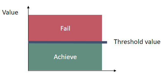
Figure 2. Schematic figure of the threshold value concept applied in the indicator.
The status evaluation is carried out and weighed against scientifically based assessment unit-specific threshold values (Table 1).
Table 2. Assessment unit specific approaches and threshold values for the shallow water oxygen indicator.
| HELCOM_ID | Assessment unit (open sea) | Approach/ method | Threshold value for concentration (mg L-1) | Threshold value for volume/ area if applied |
| SEA-001 | Kattegat | Area affected | 2, 4 and 6 mg L-1 | 1752 km2* |
| SEA-002 | Great Belt | 2, 4 and 6 mg L-1 | 348 km2* | |
| SEA-003 | The Sound | 2, 4 and 6 mg L-1 | 57 km2* | |
| SEA-004 | Kiel Bay | 2, 4 and 6 mg L-1 | 684 km2* | |
| SEA-005 | Bay of Mecklenburg | 2, 4 and 6 mg L-1 | 710 km2* | |
| SEA-006 | Arkona Basin | 2, 4 and 6 mg L-1 | 1730 km2* | |
| SEA-007B | Pomeranian Bay | Near-bottom oxygen-concentration | 4 mg L-1 (seasonally stratified) and 6 mg L-1 (well mixed) | |
| SEA-011 | Gulf of Riga | 4 mg L-1 (seasonally stratified) and 6 mg L-1 (well mixed) | ||
| SEA-013B | Gulf of Finland Eastern | Volume below the threshold | 6.0 | 14 km3 |
| SEA-014 | Åland Sea | Under development | NA | NA |
| SEA-015 | Bothnian Sea | Near-bottom oxygen-concentration | 7.7 | NA |
| SEA-016 | The Quark | 8.1 | NA | |
| SEA-017 | Bothnian Bay | 8.8 | NA | |
| * : average of areas affected by concentrations below 2, 4 and 6 mg L-1. Areas are summed for each concentration before the average over time is calculated. This means that an area with concentrations below 4 mg L-1 counts double and areas below 2 mg L-1 triples. In this way, the indicator value is a combination of severity of hypoxia and area. | ||||
3.1 Setting the threshold value(s)
The threshold value for the Eastern Gulf of Finland was based on data from 1926 to 1939. The mean 6.0 mg L-1 isoline depth in 1926-1939 was 64.1 meters corresponding to roughly 11% of the area and 2% of the volume of the Eastern Gulf of Finland. The threshold value of 14 km3 (or 4% of total volume) was fixed assuming an acceptable deviation of 100 % from the reference value of 7 km3 (Table 3).
To find the threshold value for the shallow water oxygen indicator for the Gulf of Finland Eastern, the period from 1926 to 1939 was selected and analyzed. A similar period, starting from the 1920s, was considered as a period of insignificant human influences in the HELCOM threshold-setting process (HELCOM, 2013). The mean DO = 6.0 mg L-1 isoline depth in 1926-1939 was 64.1 meters, which corresponds to roughly 11% of the area and 2% of the volume of the Gulf of Finland Eastern. The proposed threshold value of 14 km3 (or 4% of total volume) was fixed at the acceptable deviation of 100 % from the reference value of 7 km3 (Table 3).
Table 3. Proposed low oxygen limit, reference condition, acceptable deviation and threshold values for the Eastern Gulf of Finland.
| Assessment unit ID | Assessment unit | Low oxygen limit (mg L-1) | Reference condition (km3) | Acceptable deviation (%) | Threshold (km3) |
| SEA-013B | Gulf of Finland Eastern | 6.0 | 7 | 100 | 14 |
In the Gulf of Bothnia, Reference conditions were estimated for each station used in the assessment (Annex B). This was done by applying monitoring data from a relatively pre-eutrophic time-period. When data availability was inadequate, time series were extrapolated linearly back to 1940 (Figure 3). Thresholds were set assuming an acceptable deviation of 25%. Reference conditions and assessment were derived as averages of the station-specific estimates (Table 4).
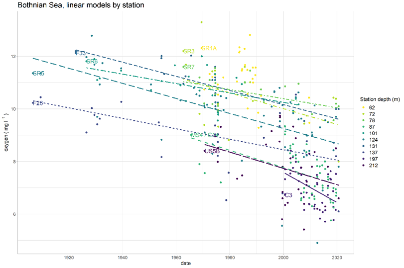
Figure 3. Long term trends in near-bottom water oxygen concentration in selected stations in the Bothnian Sea. Average slope of the station specific models was used in extrapolating the reference conditions from the present values. Lines show the significant linear trends. The labels indicate the first datapoint from each station.
The decrease in the saturation adjusted near-bottom oxygen concentration from the reference level to present (2016-2021) is estimated separately for each station (Figure 4). Acceptable deviation from the reference level has been set to 25 %. The assessment unit specific threshold is derived as the mean of the station specific values. This approach assumes that there are no changes in the monitoring station network.
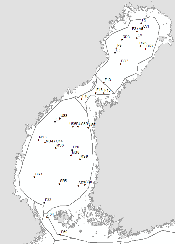
Figure 4. Map over stations included in the shallow water oxygen indicator for the Bothnian Sea, the Quark and Bothnian Bay. Approach for the Åland Sea is under development.
Reference conditions were estimated for each station used in the assessment (Annex B). This was done primarily by applying monitoring data from a relatively pre-eutrophic time-period, and when the data availability was not adequate, by extrapolating average linear trend in oxygen concentrations to the year 1940 (Figure 3). The thresholds were set with the acceptable deviation of 25% from the reference conditions, which is generally used for indicators responding negatively to increased eutrophication. The reference conditions and thresholds for the assessment units were derived as averages of the station-specific estimates (Table 4). In the indicator evaluation, monitoring data was used from those stations that were chosen for the threshold-setting.
Table 4. Proposed threshold values for application in the Gulf of Bothnia assessment units.
| Assessment unit ID | Assessment unit | Reference condition (mg L-1) | Acceptable deviation (%) | Threshold value (mg L-1) |
| SEA-015 | Bothnian Sea | 10.3 | 25 | 7.7 |
| SEA-016 | The Quark | 10.9 | 25 | 8.1 |
| SEA-017 | Bothnian Bay | 11.7 | 25 | 8.8 |
In the Western Baltic Sea, thresholds were based on pre-1970 historical data. The oldest data (1900-1909) were used to characterize the reference condition and data from the period 1950-1969 were as the target. Data from the intermediate period (1920-1939) were used to characterize a status between reference conditions and the target value (i.e. corresponding to a High-Good boundary).
A non-parametric modelling approach was used to estimate oxygen concentrations in the past. The areal extent of oxygen depletion for the period 1950-1969 was estimated at 1,652 km2. Following the approach of characterizing the first period (1900-1909) as reference condition and the later period (1950-1969) as target, threshold for oxygen depletion for HELCOM assessment units in the Danish Straits and Arkona Basin are proposed (Table 5).
For assessing the areal extent of oxygen depletion in the past, historical data prior to 1970 from the area connecting the Baltic Sea and North Sea (‘entrance area’) were obtained from the national marine monitoring database at Aarhus University. Following the approach of using different periods to characterize reference and target conditions, the oldest data (1900-1909) were used to characterize the reference condition and data from the period 1950-1969 were used to characterize the target condition. The data from the intermediate period (1920-1939) were used to characterize a status between reference conditions and the target value (i.e. corresponding to a High-Good boundary).
A non-parametric modelling approach was used to estimate oxygen concentrations in the past. The areal extent of oxygen depletion for the period 1950-1969 was estimated at 584 km2. Following the approach of characterizing the first period (1900-1909) as reference condition and the last period (1950-1969) as target, threshold for oxygen depletion for HELCOM assessment units in the Danish Straits and Arkona Basin are proposed (Table 5).
Table 5. Threshold values derived for the assessment units within the Western Baltic Sea Area.
| Assessment unit (open sea) | Approach/ method | Threshold value for concentration (mg L-1) | Threshold value for volume/ area if applied |
| Kattegat | Area affected | 2, 4 and 6 mg L-1 | 1752 km2 |
| Great Belt | Area affected | 2, 4 and 6 mg L-1 | 348 km2 |
| The Sound | Area affected | 2, 4 and 6 mg L-1 | 57 km2 |
| Kiel Bay | Area affected | 2, 4 and 6 mg L-1 | 684 km2 |
| Bay of Mecklenburg | Area affected | 2, 4 and 6 mg L-1 | 710 km2 |
| Arkona Basin | Area affected | 2, 4 and 6 mg L-1 | 1730 km2 |
In the Gulf of Riga and Pomeranian Bay, threshold values were defined as 4 mg DO L-1 and 6 mg DO L-1 for seasonally stratified (bottom depth > 15m) and well-mixed stations (bottom depth <= 15m), respectively. A concentration of 6 mg L-1 is shown to be a limit below which about 75% of fish will experience stress caused by low oxygen conditions (Vaquer-Sunyer and Duarte 2008). While growth is affected at oxygen concentrations below 6.0 mg DO L-1, other aspects of metabolism are affected at concentrations between 4 and 2 mg DO L-1 (Gray et al. 2002). Threshold values are set out in Table 6.
Table 6. Proposed threshold values for application in the Gulf of Riga and Pomeranian Bay assessment units.
| Assessment unit | Approach/ method | Threshold value for concentration (mg L-1) |
| Pomeranian Bay | Near-bottom oxygen-concentration | 4 mg L-1 (seasonally stratified) and 6 mg L-1 (well mixed) |
| Gulf of Riga | Near-bottom oxygen-concentration | 4 mg L-1 (seasonally stratified) and 6 mg L-1 (well mixed) |
4 Results and discussion
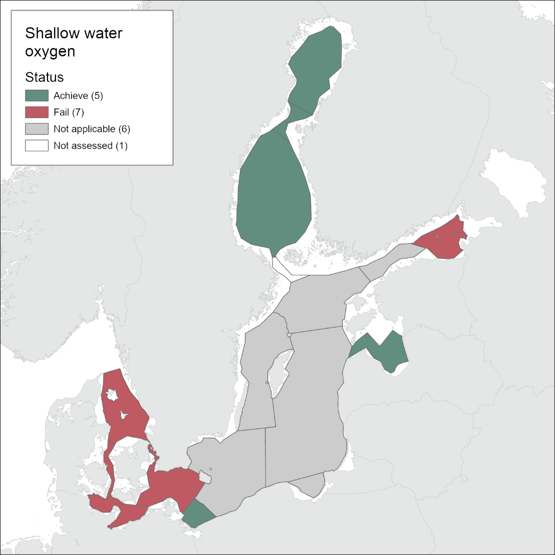
The near-bottom oxygen in shallow waters indicated good status in the Pomeranian Bay, Gulf of Riga, Bothnian Sea, The Quark and Bothnian Bay. In the Kattegat, Sound, Great Belt, Kiel Bay, Mecklenburg Bight, Arkona Sea and Gulf of Finland Eastern, status was not good. Of these, the Mecklenburg Bight and Gulf of Finland Eastern were evaluated to be in poor status (Figure 5 and table 7).
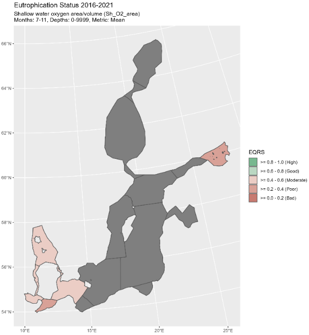
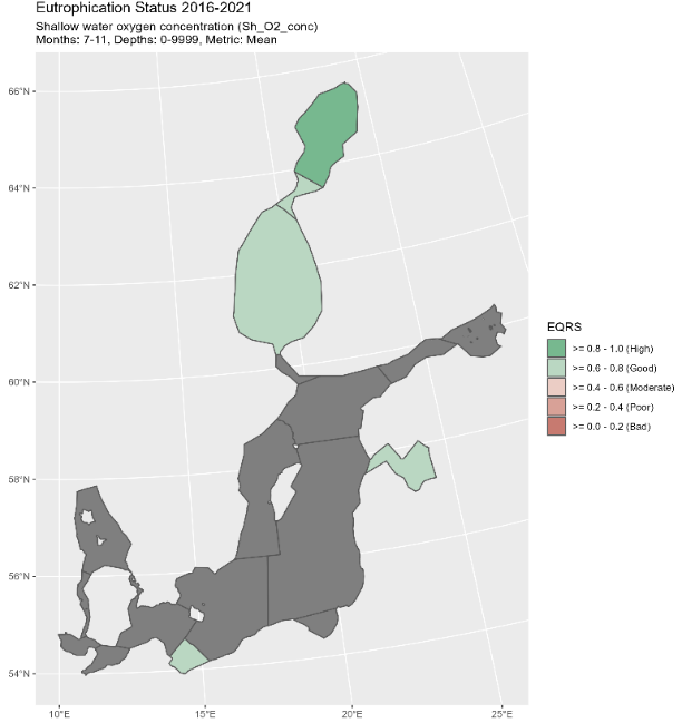
Figure 5. Map of status class. The status of the shallow water oxygen presented as Ecological Quality Ratio Scaled (EQRS). The approach applied in each assessment unit can be found in Table 7 below.
Table 7. Indicator evaluation for shallow water oxygen.
| HELCOM_ID | Assessment unit (open sea) | EQRS | Status class | Approach |
| SEA-001 | Kattegat | 0.59 | M | Area |
| SEA-002 | Great Belt | 0.54 | M | Area |
| SEA-003 | The Sound | 0.41 | M | Area |
| SEA-004 | Kiel Bay | 0.48 | M | Area |
| SEA-005 | Bay of Mecklenburg | 0.30 | P | Area |
| SEA-006 | Arkona Basin | 0.40 | M | Area |
| SEA-007B | Pomeranian Bay | 0.72 | G | Near-bottom concentration |
| SEA-011 | Gulf of Riga | 0.70 | G | Near-bottom concentration |
| SEA-013B | Gulf of Finland Eastern | 0.29 | P | Area / volume -based |
| SEA-015 | Bothnian Sea | 0.75 | G | Near-bottom concentration |
| SEA-016 | The Quark | 0.73 | G | Near-bottom concentration |
| SEA-017 | Bothnian Bay | 0.98 | H | Near-bottom concentration |
This is a pre-core indicator: the approach and threshold values are yet to be commonly agreed in HELCOM. The results are to be considered as intermediate.
4.1 Gulf of Finland Eastern
Near-bottom oxygen concentrations at stations deeper than 60 m show a declining long-term temporal trend (1906-2021) based on annual (R2 = 0.07, p <0.01, n = 782) and seasonal values from July to October (R2 = 0.16, p <0.01, n = 321) (Stoicescu et al. manuscript). Although near-bottom salinity values do not show a constant long-term trend, periods with decreasing (mid-1970s to the beginning of 1990s) and increasing (beginning of 1990s to the present) salinities can be observed. These periods are associated with distinct changes in oxygen conditions: decreasing salinity corresponds to an increase in oxygen values and vice versa. Although deep layer temperature also exhibits a fluctuating nature, as salinity and oxygen, the amplitude is smaller. Still, a clear increase in temperature is seen, especially in the last three decades (1990-2021, R2 = 0.26, p <0.01, n = 145, 0.07 degrees per year).
4.2 Gulf of Bothnia
Good status was found in the Bothnian Sea, the Quark and Bothnian Bay, with highest EQR values in the Bothnian Bay. Station specific evaluations are in Annex B.
The Gulf of Bothnia has been well oxygenated. However, oxygen in deep waters has declined over the past decades in the Bothnian Sea (1990-2012; Raateoja 2013, Ahlgren et al. 2017, Kuosa et al. 2017), and a similar though more moderate trend has been observed in the Bothnian Bay (Kuosa et al. 2017). When changes in oxygen concentration are used as a eutrophication indicator, other factors notably contributing to oxygen decline need to be considered. The decrease in oxygen concentration since 1990s has been attributed to increase in water temperature, which decreases oxygen solubility and stimulates respiration, and partly to increase in dissolved organic carbon in seawater (Ahlgren et al. 2017), as well as to strengthening stratification, which restricts the vertical oxygen supply (Raateoja 2013). Since 2000, a larger amount of Baltic Proper water, with potentially sub-saturated oxygen concentrations, has entered the deep layers of the Gulf of Bothnia, which is probably contributing to the decrease in deep-water oxygen levels (Ahlgren et al. 2017, Kuosa et al. 2017, Raateoja 2013).
4.3 Western Baltic Sea
The Western Baltic Sea is strongly affected by seasonal hypoxia and all assessment units fail to achieve good status. The situation is better in the northern parts i.e. the Kattegat and Great Belt, compared to the southwestern parts. Low oxygen concentration is to some degree a natural phenomenon in the region.
The assessment for the period 2016 to 2021 is shown in Table 8. All areas are in less than good status. However, Kattegat and Great Belt are only slight below the boundary. The Sound and Arkona Basin have affected areas just below the moderate/poor boundary bringing then in moderate condition, but just barely. Kiel Bay is in the middle of range for moderate status whereas Bay of Mecklenburg is in poor condition. The Little Belt is not assessed as the entire area is assessed within the Water Framework Directive. The overall conclusion is that the entire area is negatively affected by hypoxia, in particular the south-western part of the Western Baltic Sea.
Table 8. Results of the assessment for the period 2016-2021. All areas are the average of areas affected by oxygen concentrations below 2, 4 and 6 mg l-1, respectively. The reference condition is the estimated area between 1900 and 1909. The threshold is set to conditions (area) estimated for the period 1950-1969 (G/M). The other boundaries are found by linear interpolation. H/G: high/good status. G/M: good/moderate status. M/P: moderate/poor status. P/B: poor/bad status.
| Assessment unit ID
|
Assessment unit
|
Ref. condition
|
H/G | G/M | M/P | P/B | Worst | Status 2016 – 2021 | EQRS
2016 – 2021 |
Class |
| Area (km2) | ||||||||||
| SEA-001 | Kattegat | 0 | 876 | 1752 | 5249 | 8745 | 12241 | 1972 | 0.59 | M |
| SEA-002 | Great Belt | 0 | 174 | 348 | 782 | 1215 | 1649 | 484 | 0.54 | M |
| SEA-003 | The Sound | 0 | 28 | 57 | 125 | 193 | 261 | 123 | 0.41 | M |
| SEA-004 | Kiel Bay | 80 | 382 | 684 | 1163 | 1641 | 2120 | 967 | 0.48 | M |
| SEA-005 | Bay of Mecklenburg | 69 | 389 | 710 | 1415 | 2120 | 2825 | 1762 | 0.30 | P |
| SEA-006 | Arkona Basin | 927 | 1329 | 1730 | 3112 | 4494 | 5876 | 3094 | 0.40 | M |
It is likely that some areas had oxygen concentration less than 6 mg L -1 even in a pristine state. However, the analysis shows that moderate oxygen depletion only occurred in a very small area in the southern part of Little Belt in a pre-eutrophic state. The entire areas is sensitive to increased primary production due to excessive inputs of nutrients, primarily nitrogen, because the water column is permanently stratified, implying that oxygen is mainly supplied by advective transport in the bottom layer. This oxygen supply originates from the surface water in the Skagerrak that feeds the bottom layer and it typically reaches a minimum during August-October, when the advective transports are at their lowest and the degradation processes in sediment and bottom water are at their maximum.
4.4 Gulf of Riga
Long-term data show that deepest measured DO values stay mostly above 4 mg L-1 (Figure 6). However, in the past ~20 years, DO values below 2 ml L-1 (2.9 mg L-1), have been observed more often and a statistically significant DO decrease has been found in the Gulf of Riga, based on 2005-2018 autumn data (Stoicescu et al. 2022). From July-September data (2016-2021), values below the set threshold (4 mg L-1) have been occasionally observed in the Gulf of Riga bottom area (Figure 7).
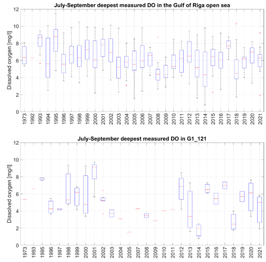
Figure 6. Boxplots of deepest measured DO in the Gulf of Riga (upper panel) and in the central station of G1/121 (lower panel) in July-September. On each box, the central mark indicates the median, and the bottom and top edges of the box indicate the 25th and 75th percentiles, respectively. The whiskers extend to the most extreme data points not considered outliers, and the outliers are plotted individually using the ‘+’ marker symbol. Please notice the different x-axis scales.
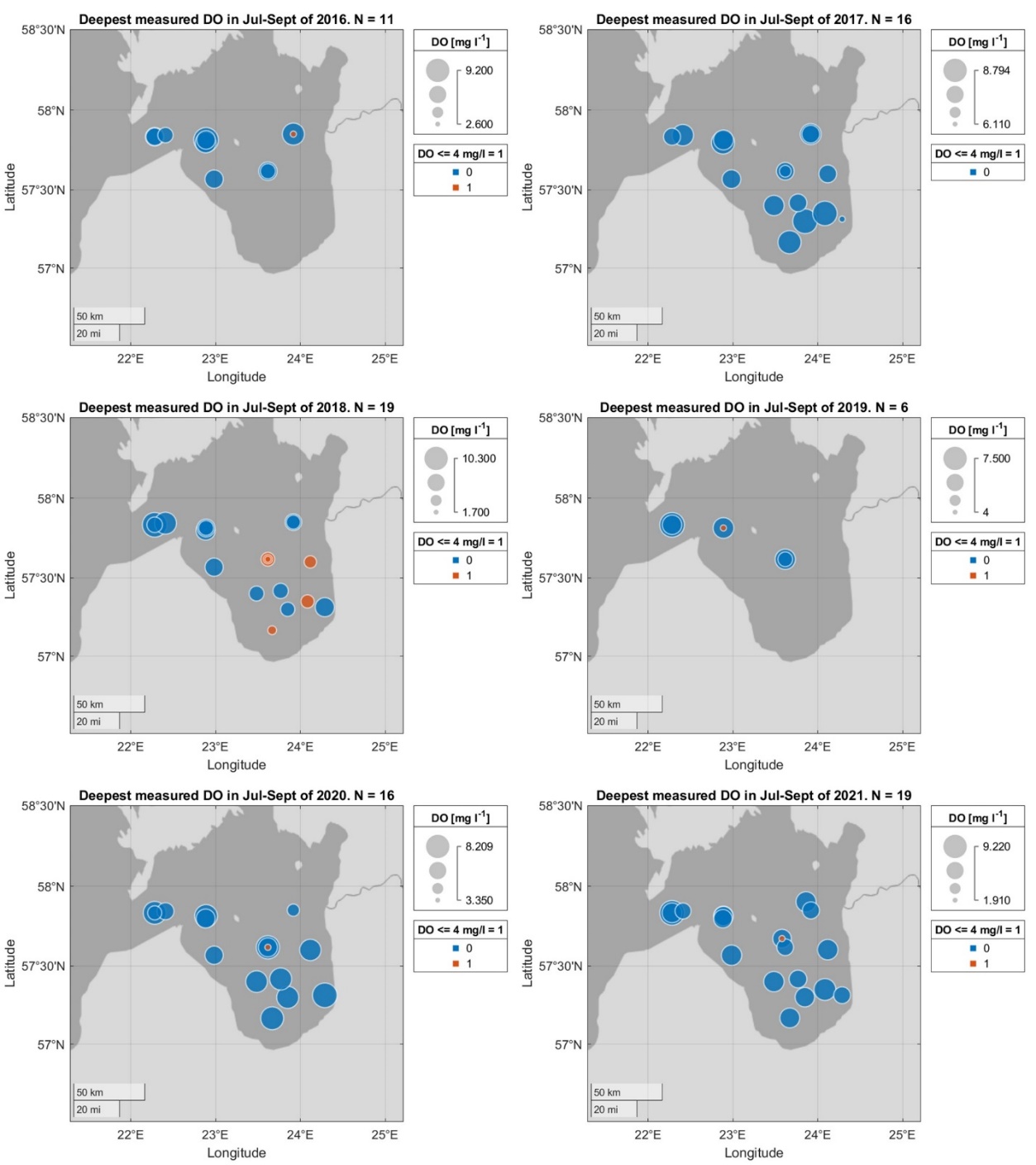
Figure 7. Deepest measured DO in the GOR area in 2016-2021 (July-September). Orange dots indicate values, where DO <= 4 mg L-1. Please notice the different scales.
Assessment period median values of station minima were generally above the 4 mg L-1 threshold with the exception of station G1/121 in the central and the deepest area of the gulf (Table 9). Stations results were weighted based on data availability. Station weights had a value of 3, if there was data from 4 or more years in the assessment period and >1 measurement per season, a weight of 1 if less data were available, and a weight of 0 if 3 years or less data were available during the assessment period. Most of the stations were assigned the weight ‘1’, three stations were given the highest weight and only one station was excluded from the overall assessment. The overall weighted mean of the station EQRs (0.70) showed that using this method, shallow water oxygen has a good status in the Gulf of Riga. Station weights are shown in Figure 8.
To determine an EQR value, the median values were scaled by giving them a value from 0 to 1, the best value of 8 mg L-1 and the worst value of 0 mg L-1 were used. The weighted mean of the scaled median had a value of 0.7, indicating good status.
Table 9. Season minimum values and assessment period median (in mg L-1, scaled values from 0 to 1) values per station.
| year/ station | 102A | 107 | 111 | 114_114A | 119 | 120 | 121A | 135 | 137A | 142 | 162B | G1_121 |
| 2016 | 2.60 | 6.20 | 4.90 | 6.05 | 4.80 | |||||||
| 2017 | 8.45 | 7.42 | 7.80 | 7.30 | 8.79 | 7.42 | 7.42 | 7.88 | 8.77 | 7.58 | 6.11 | 6.60 |
| 2018 | 2.31 | 4.10 | 4.50 | 4.80 | 4.17 | 4.67 | 3.44 | 4.48 | 3.80 | 6.14 | 6.64 | 1.70 |
| 2019 | 4.00 | 6.10 | 5.10 | |||||||||
| 2020 | 7.51 | 4.31 | 6.12 | 4.74 | 7.18 | 7.17 | 6.92 | 7.02 | 5.88 | 8.21 | 3.35 | |
| 2021 | 6.49 | 5.19 | 5.82 | 4.71 | 6.28 | 5.48 | 6.78 | 6.74 | 7.57 | 6.74 | 5.05 | 1.91 |
| Median: | 7.00 | 4.31 | 5.97 | 4.85 | 6.73 | 6.32 | 6.85 | 6.88 | 7.57 | 6.14 | 6.37 | 4.08 |
| Scaled value: | 0.87 | 0.54 | 0.75 | 0.61 | 0.84 | 0.79 | 0.86 | 0.86 | 0.95 | 0.77 | 0.80 | 0.51 |
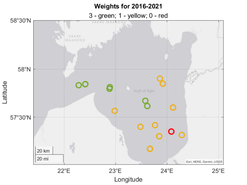
Figure 8. Weights of the stations.
4.5 Pomeranian Bay
All stations used for the oxygen assessment (Figure 9 and Table 10) are located in the shallow area of the sub-basin (<15 m) and therefore, the threshold was set to 6 mg L-1. Data in the period 2016-2021 showed that most measurements were above the threshold in the assessment season from July to November. Some individual measurements were below the threshold (predominantly in August) and only in exceptional cases the oxygen concentration was below 2 mg L-1, indicating hypoxic conditions. Assessment period median values of station minima were all above the set threshold of 6 mg L-1. Oxygen concentrations from single measurements in the northern part of Pomeranian Bay were also above the threshold in all cases, even though these stations were excluded from the assessment and only used as supporting information. Recent modelled data from the IOW (Leibniz Institute for Baltic Sea Research) support that the Pomeranian Bay is usually well-oxygenated with occasional lower values in the western part of the sub-basin. As a result, status in the Pomeranian Bay was assessed as “good”.
The Pomeranian Bay is generally well-oxygenated, but episodic events of oxygen depletion were documented in the 1990s (Powilleit et al. 1999). A combination of extraordinary meteorological and hydrological conditions together with high nutrient loads from the Odra River can cause these oxygen depletion events. Studies related to long-term changes in the benthic community indicate an increased frequency and severity of oxygen depletion events since the 1980s (Kube et al. 1998). In general, the flow pattern in the Pomeranian Bay is dominated by wind-driven circulation with easterly winds resulting in water and nutrient transport along the German coastline, while westerly winds transport nutrient rich riverine waters to the Polish coast and further eastwards. The Odra Bank is the central morphological structure of the Pomeranian Bay with depths of 7-10 m. In this area no episodic oxygen deficiencies or anoxic conditions are known and are also not expected. The deeper area of the north-eastern part of Pomeranian Bay is characterized by deep water inflows from Arkona and Bornholm Basin. Oxygen depletion is most likely to occur in the southwestern part of the sub-basin, where most monitoring stations are located.
Available data in the Pomeranian Bay was mainly located in the western and southern part of the sub-basin closer to the coast. Individual vertical profiles providing information on oxygen concentrations in the northern and deeper north-eastern part of Pomeranian Bay were not used for the assessment according to the procedure that stations with data from ≤ 3 years in the assessment period are excluded.
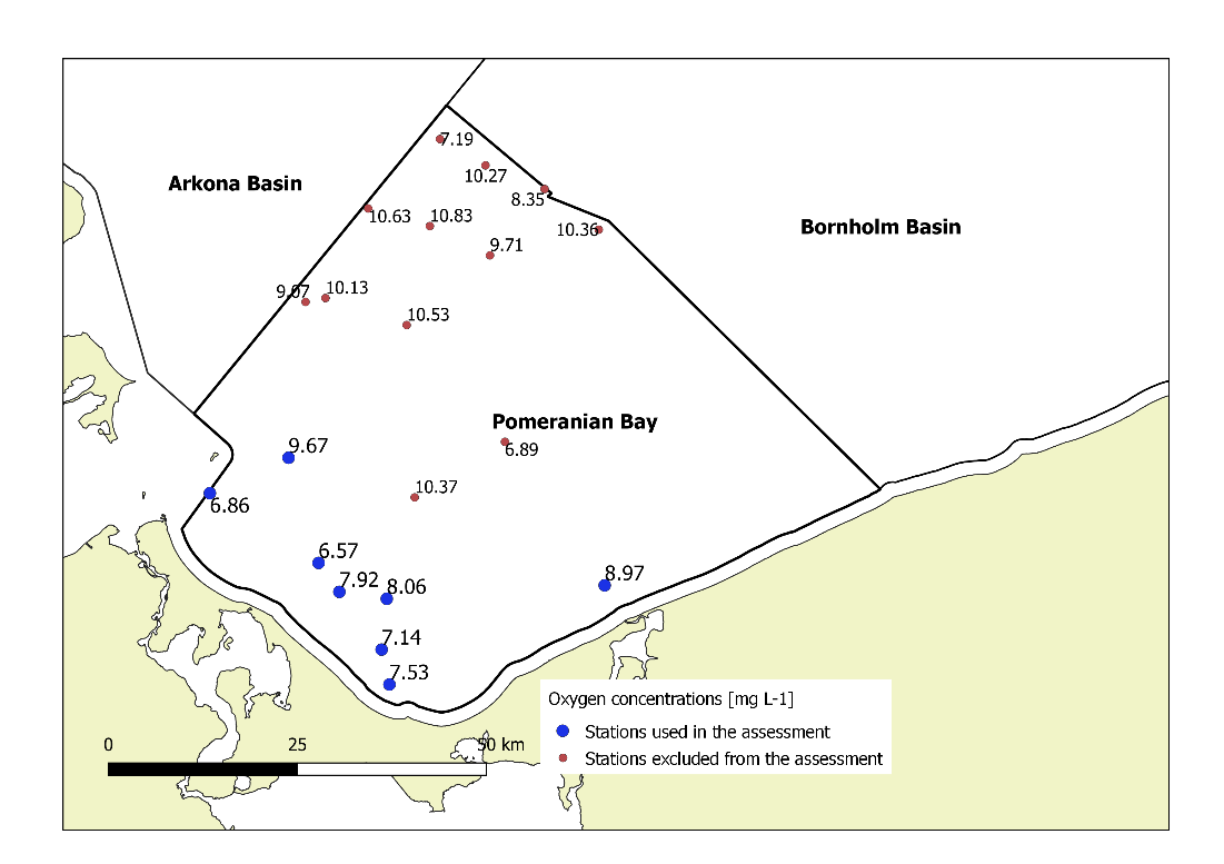
Figure 9. Oxygen concentrations (median of seasonal minima from July to November in the period 2016-2021) at stations included in the assessment (blue dots) and additional information from single measurements (orange dots) that were excluded from the assessment in the Pomeranian Bay.
Table 10. Season minimum values and assessment period median (in mg L-1, scaled values from 0 to 1) values per station.
| year/ station | OMO133 | OMTF0164 | OMOB4 | OMOB2 | BMPK14 | BMPK59 | DE-1 | OMTF0160 |
| 2016 | 7.43 | 6.57 | 5.86 | 7.63 | 9.24 | 9.27 | 7.81 | 10.43 |
| 2017 | 6.86 | 8.0 | 8.14 | 8.23 | 8.23 | 8.84 | 10.67 | |
| 2018 | 6.71 | 6.86 | 7.29 | 7.43 | 5.97 | 5.59 | 1.33 | 9.67 |
| 2019 | 7.57 | 6.29 | 7.00 | 8.14 | 7.90 | 9.10 | 8.19 | 9.43 |
| 2020 | 1.86 | 6.57 | 7.56 | 5.36 | 9.41 | 9.29 | 8.03 | 7.96 |
| 2021 | 6.60 | 6.40 | 7.33 | 7.89 | ||||
| Median: | 6.86 | 6.57 | 7.14 | 7.53 | 8.06 | 8.97 | 7.92 | 9.67 |
| EQR: | 0.57 | 0.55 | 0.60 | 0.63 | 0.67 | 0.75 | 0.66 | 0.81 |
| EQRS: | 0.66 | 0.64 | 0.68 | 0.70 | 0.74 | 0.80 | 0.73 | 0.84 |
For scaling the medians (i.e. calculation of EQR values in the range from 0 to 1), a best value of 12 mg L-1 and a worst value of 0 mg L-1 were used in relation to the threshold of 6 mg L-1. EQR values were normalized to the equidistant scale of 0.2 class width in order to use resulting EQRS values directly in the HEAT tool for integration with other indicators in the category of indirect effects.
Most of the stations were assigned the highest weight ‘3’ with data in four or more years in the assessment period and several measurements per season. Two stations were given the weight ‘1’ and two other stations with data in only two or three years were excluded from the overall assessment. The overall weighted mean of the EQRS values per station is 0.72, thus the threshold has been achieved in the Pomeranian Bay.
5 Confidence
This is a pre-core indicator. Its approach and threshold values are yet to be commonly agreed in HELCOM. The results are to be considered as intermediate.
Table 11. Confidence
| HELCOM_ID | Assessment unit (open sea) | The confidence of the AU | Confidence coming from data in percentages | Confidence coming from threshold in percentages |
| SEA-001 | Kattegat | |||
| SEA-002 | Great Belt | |||
| SEA-003 | The Sound | |||
| SEA-004 | Kiel Bay | |||
| SEA-005 | Bay of Mecklenburg | |||
| SEA-006 | Arkona Basin | |||
| SEA-007 | Bornholm Basin | |||
| SEA-007B | Pomeranian Bay | moderate | ||
| SEA-008 | Eastern Gotland Basin | |||
| SEA-009 | Gdansk Basin | |||
| SEA-010 | Western Gotland Basin | |||
| SEA-011 | Gulf of Riga | 75 | 50 | 100 |
| SEA-012 | Northern Baltic Proper | |||
| SEA-013A | Gulf of Finland Western | |||
| SEA-013B | Gulf of Finland Eastern | 50 | 50 | 50 |
| SEA-014 | Åland Sea | |||
| SEA-015 | Bothnian Sea | |||
| SEA-016 | The Quark | |||
| SEA-017 | Bothnian Bay |
5.1 Confidence for the Gulf of Finland Eastern
The confidence of the indicator is assessed according to Fleming-Lehtinen et al. (2015), taking into account the temporal and spatial resolution of the data and the confidence of the indicator threshold. The confidence of the indicator in the eastern Gulf of Finland area for the assessment period 2016-2021 was 50% (50% for data and 50% for the threshold).
5.2 Confidence for the Gulf of Bothnia
No assessment has been made.
5.3 Confidence for the Western Baltic Sea
A model approach for assessing the distribution of severe and moderate oxygen depletion has been established for the Danish Straits and the Arkona Basin. This model approach, which is based on analyzing oxygen profiles from monitoring cruises within a restricted time windows during the critical period in late summer and autumn, is well tested and has been applied for 20 years. The proposed methodology relies on a good data coverage, and it is to be tested if it can be applied for other basins. In basins with a less complicated bottom typography, it might be possible to apply the technique with fewer data than used here. However, this must be tested for each basin. In basins with higher oxygen concentrations and hence no immediate problems with oxygen depletion, e.g., the North-Eastern parts of the Baltic Sea, the methodology can still be used to assess the status if higher oxygen concentrations, e.g. 6 or 8 mg L-1 are used to define the areas.
5.4 Confidence for the Gulf of Riga
The confidence of the indicator is assessed according to Fleming-Lehtinen et al. (2015), considering the temporal and spatial resolution of the data and the confidence of the indicator threshold. The confidence of the indicator in the Gulf of Riga area for the assessment period 2016-2021 was 75% (50% for data and 100% for the threshold).
5.5. Confidence for the Pomeranian Bay
The overall confidence of shallow water oxygen in the Pomeranian Bay is assessed as moderate. Following the confidence rating approach used for other indicators of the eutrophication assessment (e.g. nutrients, chlorophyll), different aspects for temporal and spatial confidence as well as accuracy and methodological confidence were considered. The temporal confidence takes account of the number of annual observations and the continuity of observations during the assessment season (possibly missing months). Both temporal aspects were assessed as high based on the number of annual observations > 20 (confidence class boundaries of chlorophyll were used for oxygen as well) and observations in all months of the assessment season per year. Although individual years were assessed as moderate due to annual observations < 20, the overall temporal confidence was still high. Spatial confidence was assessed as low, because less than 60% of the area was sampled per year, leaving a large part of Pomeranian Bay without monitoring and without substantial information on oxygen concentrations. Although a large part of the assessment area is not monitored, or at least not monitored frequently, it is reasonable to assume that given the characteristics of the assessment area being shallow, exposed, and well-mixed, the results are valid for a larger area than sampled within 10 and 15 meters. In particular, measurements in the shallow area of the Odra Bank, where no oxygen deficiency is expected, would probably improve the assessment result if regularly monitored. The accuracy was estimated as high, because all EQRS values were clearly above the threshold, even if no exact calculation of the variable confidence level was done to estimate the probability of classification of being above or below the threshold. Methodological confidence was assessed as high based on the quality of monitoring according to HELCOM guidelines and quality assured data. Combining the different aspects similar to the procedure as applied in the HEAT tool for other indicators resulted in a moderate confidence for the shallow water oxygen assessment in the Pomeranian Bay.
6 Drivers, Activities, and Pressures
Oxygen depletion is an indirect effect of eutrophication having an indirect link to anthropogenic pressures, through increased anthropogenic nutrient loads and subsequent increase of organic matter sedimentation.
For HOLAS 3 initial work has been carried out to explore Drivers (and driver indicators) to evaluate how such information can be utilised within the DAPSIM management frameworks. It is recognised that only a small portion of the drivers via proxies such as relevant human activities have been addressed for eutrophication assessment. Wastewater treatment (Drivers and driver indicators for Wastewater Treatment) and agriculture (Drivers and driver indicators for Agricultural Nutrient Balance) have been explored in these pilot studies for HOLAS 3.
Diffuse sources constitute the highest proportion of total nitrogen (nearly 50%) and total phosphorus (about 56%) inputs to the Baltic Sea (HELCOM 2022). For total nitrogen, atmospheric deposition on the sea has the second highest share (24%) followed by natural background loads (20%) and point sources (9%). Natural background loads have the second highest share of total phosphorus inputs to the Baltic Sea (20%), followed by point sources (17%) and atmospheric deposition (7%). Point sources include activities such as municipal wastewater treatment plants, industrial plants and aquacultural plants and diffuse sources consists of anthropogenic sources as agriculture, managed forestry, scattered dwellings, storm water etc.
A significant reduction of nutrient inputs has been achieved for the whole Baltic Sea. The normalized total input of nitrogen was reduced by 12% and phosphorus by 28 % between the reference period (1997-2003) and 2020 (HELCOM 2023). The maximum allowable input (MAI) of nitrogen in this period was fulfilled in the Bothnian Bay, Bothnian Sea, Danish Straits and Kattegat and the maximum allowable input of phosphorus in the Bothnian Bay, Bothnian Sea, Danish Straits and Kattegat.
Further developing an overview of such components and the relevant data to be able to better quantify the linkages within a causal framework provide the opportunity for more informed management decisions, for example targeting of measures, and can thereby support the achievement of Good Environmental Status.
Table 12. Brief summary of relevant pressures and activities with relevance to the indicator.
| General | MSFD Annex III, Table 2a | |
| Strong link | Substances, litter and energy
– Input of nutrients – diffuse sources, point sources, atmospheric deposition |
|
| Weak link | Substances, litter and energy
– Input of organic matter – diffuse sources and point sources |
7 Climate change and other factors
The current knowledge of the effects of climate change on eutrophication is summarized in the HELCOM fact sheet for climate change (HELCOM and Baltic Earth 2021). The effect of climate change on the nutrient pools is not yet separable from the other pressures, and the future nutrient pools will dominantly be affected by the development of nutrient loading. Climate change is, with medium confidence, considered to increase the stratification, further exacerbating near-bottom oxygen conditions and increase the internal nutrient loading. (HELCOM and Baltic Earth 2021).
7.1 Gulf of Finland
Due to the openness of the basin with no major sills on the western border, the deep layer of the Gulf of Finland is strongly influenced by lateral advection of more saline and low-oxygen water from the Northern Baltic Proper. The east-west spread of the deep layer depends strongly on wind patterns and Major Baltic Inflows (e.g. Alenius et al. 2016; Lehtoranta et al. 2017). A permanent halocline exists in the western and central area of the gulf (Alenius et al. 1998) although it can disappear in the winter under certain meteorological conditions (Liblik et al. 2013; Lips et al. 2017). The eastern part of the gulf is also influenced by the spread of saline water from the west, but here no permanent halocline exists. The surface layer of the eastern Gulf of Finland is affected by freshwater discharge from the river Neva (Alenius et al. 1998). Nutrient inputs from river Neva exceed the maximum allowable inputs (HELCOM 2023), meaning the basin is still under strong anthropogenic influences.
July to October near-bottom oxygen saturation values from stations 60 metres deep or deeper indicate that during the last 116 years, oxygen saturation concentration has decreased by 0.57 mg L-1 (R2 = 0.10, p <0.01, n = 288, Stoicescu et al. manuscript). Oxygen saturation decreases from 1993 to 2021 were even steeper, 0.97 mg L-1 (R2 = 0.28, p <0.01, n = 147). Using regular monitoring data, the 1993-2021 average per cent of water volume under low oxygen conditions was roughly 12%. Considering the found oxygen saturation decrease (0.97 mg L-1 from 1993 to 2021) – 0.97 mg L-1 was added to monitored DO data – it was estimated that the average volume of low DO waters, was roughly 8% – so a 4% increase in the volume of low DO waters could be attributed to increasing temperature.
7.2 Western Baltic Sea
The effects of a future warmer climate were analyzed in Bendtsen and Hansen (2012). Increasing temperature lowers the solubility of oxygen and hence the transport of oxygen with inflowing bottom water, where oxygen concentration is governed by the concentration in the surface water of Skagerrak. In addition, higher a temperature will stimulate the degradation of organic matter and thereby increase oxygen consumption. The results in Bendtsen and Hansen (2012) show that the latter is about four times more important than the lowering of oxygen solubility. It also shows that a significant increase in the area affected by low oxygen concentrations and the duration of the period is to be expected.
These direct effects of higher temperature are quite certain. In addition, there may be changes in run off and hence nutrient input, changes in primary production and the food web and effects on water column stratification. These effects are uncertain and cannot be quantified today.
7.3 Gulf of Riga
The Gulf of Riga is a seasonally stratified shallow basin which is fully mixed in winter. The majority of water exchange takes place via the Irbe Strait in the west, from where the gulf’s deep waters can be renewed in summer by inflows of saltier water from the eastern Baltic Proper over the sill (Lips et al. 1995). Stratification is strongest in the years with the highest summer surface temperature and spring river discharge Skudra and Lips (2017). Stoicescu et al. (2022) suggested that a sequence of certain processes (earlier developed and long-lasting haline stratification in the deep layer, large river inflow, strong thermal stratification, low winds, longer productive season) could trigger extensive hypoxic events in the Gulf of Riga. Based on the projections of meteorological and hydrological conditions (HELCOM and Baltic Earth 2021), the frequency and extent of hypoxia will likely increase in the future (Stoicescu et al. 2022).
7.4 Bothnian Bay
The Bothnian Bay is separated from the Baltic Proper by the Archipelago Sea and a sill in the Åland Sea. These prevent deep water inflow to the basin, and therefore the deep water does not become anoxic. There does, however, exist a salinity stratification, that has become stronger due to decreased surface salinity. This has decreased the ventilation of the deep water, and may be a cause behind the decrease in near-bottom oxygen concentration.
8 Conclusions
8.1 Future work or improvements needed
The indicator is in test use in HOLAS 3, with an aim of developing it toward core indicator status by HOLAS 4. The development work includes potentially combining and harmonizing the approaches used in different assessment units. In addition, it may be relevant to explore development in other sub-basins where the oxygen debt indicator is also applied (should shallow waters in those basins be relevant to assess) with spatial integration of the two indicators as a subsequent step. The current pre-core indicator addresses a significant issue both from a policy and ecological perspective and is also relevant due to its links with benthic habitats so harmonisation and further development beyond HOLAS 3 would be valuable.
9 Methodology
9.1 Approach for the Gulf of Finland Eastern
To develop a shallow-water oxygen indicator for the Gulf of Finland Eastern, all available oxygen water sample analyses from the area were gathered from several databases resulting in a dataset from 1900 until 2021 (Stoicescu et al. manuscript). A volume-based approach was applied and a concentration of DO <= 6 mg L-1 was selected, to characterize the water volume under low oxygen conditions. This concentration is shown to be a limit below what about 75% of fish will experience stress caused by low oxygen conditions (Vaquer-Sunyer and Duarte, 2008).
To find the volume estimate, a mean profile was compiled for each year in the assessment period. The DO = 6 mg L-1 isoline depth was found for each of these mean profiles, and the average depth for the current assessment period was used for the volume estimate (Stoicescu et al. manuscript).
Because the (eastern) Gulf of Finland is strongly affected by deep-layer advection of saltier and deoxygenated waters, a salinity correction of oxygen concentrations was proposed. This would remove the hydrography effects from the indicator results and allow the estimation of the anthropogenic factor influencing the oxygen conditions.
By knowing the salinity values from a period of low or no human influence (the chosen reference period, 1926-1939), current salinity values, and the long—term relationship between salinity and oxygen, we can predict current oxygen values, which could occur under minimum anthropogenic influences / which would correspond to reference period salinities (Stoicescu et al. manuscript). Correcting oxygen to salinity gives higher adjusted DO values (compared to measured DO), when the measured salinity is higher than the depth group’s average salinity from the reference period. Higher adjusted DO values, compared to measured DO, move the minimum depth, where DO = 6 mg L-1, deeper in the water column (decreasing the area and volume), thus removing the effect of hydrography from the assessments.
Formula used to find adjusted DO values:
![]()
O2 measured = measured oxygen
slopegi = slope of the linear model for depth group i
Sref = average salinity for the depth group i in the reference period (1926-1939)
S = measured salinity
Table 12. Linear model results (all available data) and average salinities (reference period data) by depth group, using data from July- October. Mean SP – average salinity (PSU) of the depth group. O2 gi = average oxygen. slopegi = slope of the linear model. intgi = intercept of the linear model, Sref – 1926-1939 average salinity of the depth group.
| ≥ | < | July-October | July-October | ||||
| group | Min dep | Max dep | intgi | slopegi | O2 gi | Mean SP | Sref |
| g30 | 27.5 | 32.5 | 11.45 | -0.54 | 8.46 | 5.53 | no data |
| g35 | 32.5 | 37.5 | 13.66 | -0.96 | 8.01 | 5.87 | 4.25 |
| g40 | 37.5 | 42.5 | 13.64 | -0.97 | 7.52 | 6.28 | 4.83 |
| g45 | 42.5 | 47.5 | 16.74 | -1.50 | 6.83 | 6.61 | 6.62 |
| g50 | 47.5 | 52.5 | 16.00 | -1.44 | 6.01 | 6.94 | 6.81 |
| g55 | 52.5 | 57.5 | 15.55 | -1.47 | 4.87 | 7.27 | 7.04 |
| g60 | 57.5 | 62.5 | 15.52 | -1.47 | 4.27 | 7.66 | 7.46 |
| g65 | 62.5 | 67.5 | 15.83 | -1.54 | 3.40 | 8.08 | 7.50 |
| g70 | 67.5 | 72.5 | 14.38 | -1.43 | 2.46 | 8.35 | 7.51 |
| g75 | 72.5 | 999 | 12.96 | -1.29 | 1.87 | 8.57 | 8.49 |
Besides salinity, temperature also affects the oxygen conditions in the water. Climate change related increasing water temperature decreases oxygen solubility, which in turn raises the upper boundary of low-oxygen waters. Short-term temperature changes could be affected by deep-layer advection, but the long-term changes are driven by climate change. Although, the increase in temperature has not been taken into account in the indicator methods, the influence of decreased oxygen solubility on the boundary depth of low-DO waters can be estimated.
To define the volume of low-oxygen waters, we found 6 mg DO L-1 isoline depths on yearly average profiles (according to Stoicescu et al. manuscript). The yearly mean profile was found by averaging monthly mean profiles, which were compiled based on all available data in the Gulf of Finland Eastern, within a month/year. To ensure all possible data would be included, we populated the measured profiles of water samples analyses with data at standard depths (10-meter interval) by linearly interpolating oxygen values.
Using data from 2016-2021, yearly mean profiles were constructed and DO isoline 6 mg L-1 depths found, which put the shallowest isoline depth at 35.3m (2019) and deepest at 50.4m (2018).
Yearly DO = 6 mg L-1 isoline depths were used to find the area and volume estimates of low oxygen waters in the Gulf of Finland Eastern. The area and volume estimates were found using EMODnet Bathymetry data (https://portal.emodnet-bathymetry.eu/).
When applying the developed methods to the most recent data, we found an example assessment period result of 43.9 m, which represents an average depth, where DO = 6.0 mg L-1. To estimate the change in results when removing hydrography effects, we adjusted the 2016-2021 data to salinity and found the DO = 6.0 mg L-1 isoline depths and corresponding areas and volumes. From the results, it is seen that adjusting DO to salinity lowers the volume estimates, on average, roughly 2.9% (Table 13, from Stoicescu et al. manuscript).
Table 13. Comparison of monitored oxygen (DO) and salinity adjusted oxygen (DO_adj) results.
| DO = 6.0 mg L-1 depth (m) | Area (km2) | Area (%) | Volume (km3) | Volume (%) | ||
| 2016 | DO | 41.0 | 4651.1 | 52.5 | 68.8 | 18.5 |
| DO_adj | 45.0 | 3975.4 | 44.9 | 51.5 | 13.8 | |
| 2017 | DO | 41.4 | 4594.4 | 51.9 | 67.1 | 18.0 |
| DO_adj | 44.0 | 4156.4 | 47.0 | 55.7 | 14.9 | |
| 2018 | DO | 50.4 | 3108.7 | 35.1 | 32.5 | 8.7 |
| DO_adj | 51.0 | 3023.8 | 34.2 | 30.8 | 8.3 | |
| 2019 | DO | 35.3 | 5607.0 | 63.3 | 97.9 | 26.3 |
| DO_adj | 39.0 | 4967.7 | 56.1 | 78.4 | 21.1 | |
| 2020 | DO | 49.4 | 3263.8 | 36.9 | 35.8 | 9.6 |
| DO_adj | 51.5 | 2942.8 | 33.2 | 29.3 | 7.9 | |
| 2021 | DO | 45.6 | 3860.3 | 43.6 | 49.2 | 13.2 |
| DO_adj | 47.8 | 3500.6 | 39.5 | 41.2 | 11.1 | |
| 20162021 | DO | 43.9 | 4180.9 | 47.2 | 58.6 | 15.7 |
| 20162021 | DO_adj | 46.4 | 3761.1 | 42.5 | 47.8 | 12.8 |
9.2 Approach for the Gulf of Bothnia
The approach used for the shallow water oxygen indicator in the Bothnian Bay, Quark and Bothnian Sea is concentration-based. In these areas, oxygen hypoxia has not occurred, but oxygen concentrations have decreased. In order to account for the deteriorating development, the indicator is based on changes in near-bottom oxygen concentration from the reference period.
The indicator estimates the temporal change in near-bottom oxygen concentration in July – October, when the oxygen concentrations are lowest, from the reference period to the assessment period. In order to exclude the effect of increasing temperature on oxygen solubility from the observed negative trends in oxygen concentration, the oxygen concentrations were first transformed to oxygen saturation as described in HELCOM COMBINE manual, and the oxygen saturation values where then calculated back to “saturation corrected oxygen concentrations” using oxygen solubility at site specific average near-bottom temperatures and salinities. The effect of saturation correction was small, but consistent (Annex B).
9.3 Approach for the Western Baltic Sea
Since 2002, a spatial interpolation model has been used to assess the areal distribution of low oxygen concentrations in this area (HELCOM 2003). The model has been undergoing minor modifications since the original version, but the overall approach has remained the same. Furthermore, the latest version of the model has been applied to oxygen profile data from 1989 to 2021. Before 1989, the availability of CTD casts limits the applicability of the model and therefore, the areal extent of low oxygen concentrations has not been compiled for these earlier years.
CTD profiles within a restricted period (not more than 15 days) are analyzed to determine the depths in the profile where the oxygen concentration fall below certain thresholds (2 and 4 mg/l) or estimate the depths where these threshold concentrations may have been reached in case oxygen concentrations below the threshold values are not observed within the profile (Methodology figure 1). In the latter case, the deeper part of the oxygen profile is extrapolated if measured oxygen concentrations are close to the thresholds, ensuring that the oxygen profile is not extrapolated too far beyond the measured profile. When such depth estimates cannot be obtained, default values are produced as function of the station depth. This approach ensures that the information from all oxygen profiles is used, whether these represent oxygen depleted, deficient or replete conditions. These depths, representing oxygen concentration thresholds (z2 and z4), are point observations in space (x,y) and subsequently interpolated spatially using Ordinary Kriging. This spatial interpolation method estimates the depth in a given point (xpred,ypred) through a weighted average of the discrete profile observations (xobs,i, yobs,i; i=1…n), where weights are determined from the Euclidian distance between the prediction point and the observed profiles. This means that depths (z2 and z4) from observation points closer to the prediction point (xpred,ypred) are given higher weight than depths from observations points farther away. Since the Danish Straits have a complex morphology with three main connections between the Arkona Basin and the Kattegat, a segmented spatial interpolation is implemented to reduce interpolation across land. Furthermore, for interpolating across the two sills to the Arkona Basin ‘pseudo stations’ are placed on both sides of the sill with oxygen threshold depths (z2 and z4) replicated from the nearest station with measured oxygen profile. This modification is implemented to better capture the effect that there are two basins on each side of the sill with different oxygen conditions, i.e. avoiding a too smooth interpolation across the sills. For more details on the algorithm and the spatial interpolation, see HELCOM (2003) and Rytter et al. (2021).
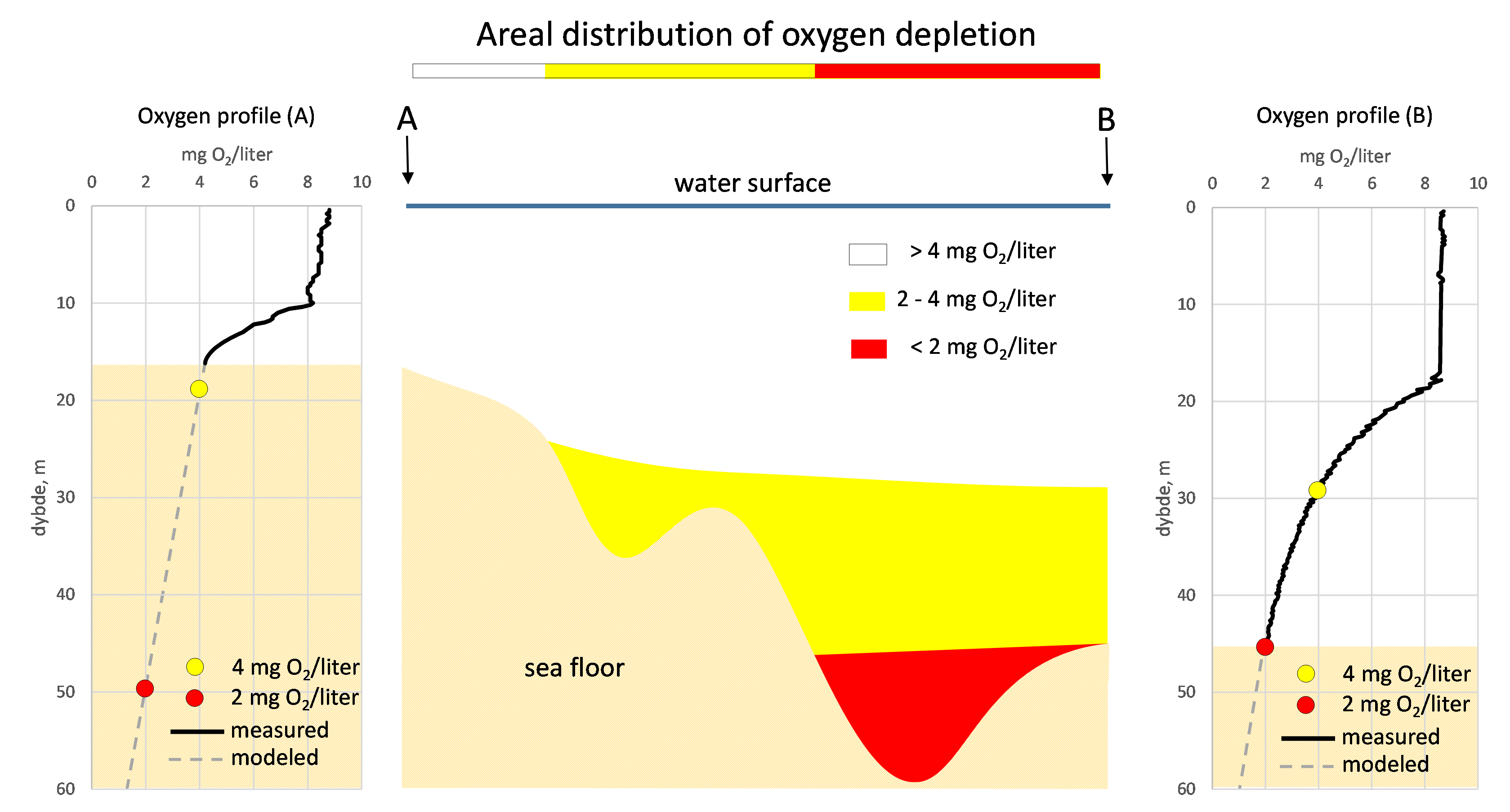
Figure 10. Illustration of the spatial interpolation model with two profiles, one with oxygen thresholds measured within the profile and one with oxygen thresholds estimated by extrapolation of the deeper part of the profile. These depths are then interpolated spatially using Ordinary Kriging with spatial restrictions to reduce interpolation across land and sills.
This document describes an approach using a spatial interpolation model to assess the areal distribution of low oxygen concentrations developed by Aarhus University and tested in the western Baltic Sea. The contents of this document are based on expert input from Aarhus University, and do not necessarily reflect an official Danish position on the indicator.
The approach draws on an oxygen debt indicator which was developed for the Baltic Sea Action Plan (HELCOM 2013) covering the Bornholm Basin and the Gotland Basin, both basins characterized by perennial hypoxia. No HELCOM indicator has been developed yet for the shallow coastal areas. These include the entrance area to the Baltic Sea (the Danish Straits, including the Kattegat, the Belt Sea, the Sound, the western Baltic Sea, Kiel Bay and Bay of Mecklenburg and the Arkona Basin), areas in the North Eastern parts of the Baltic Sea and enclosed areas like Riga Bay. In this area, hypoxia is seasonal, typically peaking with the largest areal distribution in September. This document proposes an oxygen indicator for the entrance area to be applied in HELCOM HOLAS 3.
9.4 Approach for the Gulf of Riga and Pomeranian Bay
For the Gulf of Riga open sea area and the Pomeranian Bay, an oxygen minima approach, based on the methods developed by Germany, was proposed. This approach is based on the deepest measured oxygen values near the sea bottom (a rule was applied, that the deepest measured value had to be close to the sea bottom, maximum 4 m from the bottom). The simple outline of the indicator is that every station gets an oxygen value and a weight for the assessment, then the assessment area result is found based on these station specific oxygen values and weights. The oxygen value of a station is found as a median value of station minimum values in the assessment period. The minimum values are found for a predefined season for every year.
Weights assigned to stations depend on data availability and the method is based on the method used in Pomeranian Bay of the indicator. Weight ‘3’ was assigned to stations with data from 4 or more years in the assessment period and >1 measurement per season. Weight ‘1’ was assigned to stations with less data than specified above. Weight ‘0’ was given to stations with data from ≤ 3 years in the assessment period, meaning that these data were excluded and not considered in the assessment.
The proposed thresholds of 4 mg DO L1 and 6 mg DO L-1, are set separately for seasonally stratified stations (bottom depth > 15m) and well-mixed stations (bottom depth <= 15m), respectively.
For Gulf of Riga and the Pomeranian Bay, the results are presented as assessment period median values of station minima values. The weighted mean of these median values gives the assessment area result, which is presented as EQRS (scaled ecological quality ratio, from 0 to 1).
10 Data
Result: Shallow water oxygen
10.1 Data applied in the Gulf of Finland
To test the proposed shallow water oxygen indicator in the eastern part of the Gulf of Finland, all available data from ICES, VESLA, Gulf of Finland Year database and Estonian environmental database (KESE) were pooled, and a core dataset (mostly water samples) ranging from 1900-2021 was compiled for further analysis (Stoicescu et al. manuscript).
10.2 Data applied in the Gulf of Bothnia
The analyses are based on data retrieved from Swedish Sharkweb database and Finnish Vesla database and complemented with data from ICES database, where oxygen profiles were missing from the two national databases. This mainly concerned data before 1960es. ICES data was attributed to HELCOM hydrographical monitoring stations, retrieved from HELCOM map and data service, using a buffer zone with diameter of 2 nautical miles, following the quality standard for open sea CTD monitoring.
10.3 Data applied in the Western Baltic Sea
10.4 Data applied in the Gulf of Riga
For the oxygen minima indicator testing and background analysis, all available water sample analysis data were gathered from Estonian environmental database (KESE), and provided by Latvia. Deepest measured July to September data from the open sea data area were available mainly from the beginning of 1990s to present day, with the exception of 1973 (Figure 11).
Figure 11. Deepest measured (maximum 4 m from bottom) water sample data availability from the Gulf of Riga open sea area in July to September.
For scaling the medians (i.e. finding the EQR by giving them a value from 0 to 1), the best value of 8 mg L-1 and the worst value of 0 mg L-1 were used. This information was utilised for the weighting (Data table 1 and Figure 9).
Table 14. Season data count per station and weights for the assessment period.
| year/station | 102A | 107 | 111 | 114_114A | 119 | 120 | 121A | 135 | 137A | 142 | 162B | G1_121 |
| 2016 | 2 | 3 | 3 | 1 | 2 | |||||||
| 2017 | 1 | 2 | 2 | 2 | 1 | 1 | 1 | 1 | 1 | 1 | 1 | 2 |
| 2018 | 1 | 2 | 3 | 3 | 1 | 1 | 1 | 1 | 1 | 1 | 1 | 3 |
| 2019 | 2 | 2 | 2 | |||||||||
| 2020 | 1 | 1 | 2 | 3 | 1 | 1 | 1 | 1 | 1 | 1 | 3 | |
| 2021 | 1 | 2 | 3 | 3 | 1 | 1 | 1 | 1 | 1 | 1 | 1 | 3 |
| Weights: | 1 | 1 | 3 | 3 | 1 | 1 | 1 | 1 | 0 | 1 | 1 | 3 |
10.5 Data applied in the Pomeranian Bay
For the shallow water oxygen assessment in the Pomeranian Bay, all available data were taken from the ICES database. Most of the station names were taken from the ICES station dictionary, only one station was named otherwise (DE-1). Data from July to November were considered for the assessment using deepest measurements (maximum 4 m from bottom). As most of the stations are shallow (< 15 m), the maximum from bottom was predominantly less than 2 m for the deepest measurement (Figure 12).
Figure 12. Location of the stations used for the shallow water oxygen assessment in the Pomeranian Bay.
Table 15. Season data count per station and weights for the assessment period.
| year/ station | OMO133 | OMTF0164 | OMOB4 | OMOB2 | BMPK14 | BMPK59 | DE-1 | OMTF0160 |
| 2016 | 5 | 5 | 8 | 3 | 3 | 3 | 1 | 1 |
| 2017 | 2 | 2 | 5 | 3 | 3 | 3 | 1 | |
| 2018 | 4 | 3 | 6 | 3 | 3 | 3 | 2 | 1 |
| 2019 | 3 | 3 | 6 | 3 | 3 | 3 | 1 | 1 |
| 2020 | 1 | 1 | 4 | 3 | 3 | 3 | 2 | 3 |
| 2021 | 3 | 3 | 3 | 3 | ||||
| Weights: | 3 | 3 | 3 | 3 | 3 | 3 | 1 | 1 |
Weights were assigned accordingly:
3 – If there was data from 4 or more years in the assessment period and >1 measurement per season
1 – Less data than specified above
0 – Data from ≤ 3 years in the assessment period
Weighted mean of the scaled median (EQRS value):
July-November: 0.72
11 Contributors
Vivi Fleming , Laura Hoikkala , Lena Viktorsson, Philip Axe, Emilie Breviere, Stella-Theresa Stoicescu , Urmas Lips, Birgit Heyden, Wojciech Krasniewski; Jacob Carstensen, Lasse Tor Nielsen, Stiig Markager.
HELCOM Secretariat: Laura Kaikkonen, Joni Kaitaranta, Theodor Hüttel, Owen Rowe.
12 Archive
This version of the HELCOM core indicator report was published in April 2023:
The current version of this indicator (including as a PDF) can be found on the HELCOM indicator web page.
There are currently no earlier versions of this indicator.
13 References
Ahlgren, J., Grimvall, A., Omstedt, A., Rolff, C. & Wikner, J. 2017. Temperature, DOC level and basin interactions explain the declining oxygen concentrations in the Bothnian Sea. Journal of Marine Systems 170: 22–30.
Alenius, P., Myrberg, K., Roiha, P., Lips, U., Tuomi, L., Pettersson, H., Raateoja, M. 2016. Gulf of Finland physics. In Raateoja, M., Setälä, O. (eds): The Gulf of Finland assessment. Reports of the Finnish Environment Insitute 27:2016.
Bendtsen, J. & Hansen, J. 2012. Effects of global warming on hypoxia in the Baltic Sea-North Sea transition zone. Ecological Modelling 264: 17-26.
Conley, D.J., Carstensen, J., Ærtebjerg, G., Christensen, P.B., Dalsgaard, T., Hansen, J.L.S., Josefson, A.B. (2007) Long-term changes and impacts of hypoxia in Danish coastal waters. Ecol. Appl. 17: S165-S184. https://doi.org/10.1890/05-0766.1
EU. 2000. DIRECTIVE 2000/60/EC OF THE EUROPEAN PARLIAMENT AND OF THE COUNCIL of 23 October 2000 establishing a framework for Community action in the field of water policy (Water Framework Directive). Official Journal of the European Union, L 327/2, 22.12.2000.
EU. 2008. Directive 2008/56/EC of the European Parliament and the Council of 17 June 2008 establishing a framework for community action in the field of marine environmental policy (Marine Strategy Framework Directive). Official Journal of the European Union, L 164/19, 25.06.2008.
Fleming-Lehtinen, V., Andersen, J. H., Carstensen, J., Łysiak-Pastuszak, E., Murray, C., Pyhälä, M. & Laamanen, M. (2015). Recent developments in assessment methodology reveal that the Baltic Sea eutrophication problem is expanding. Ecological Indicators 48, 380–388.
Gray, John S., Rudolf Shiu-sun Wu, Ying Ying Or (2002) Effects of hypoxia and organic enrichment on the coastal marine environment. MEPS 238:249-279 – doi:10.3354/meps238249
HELCOM (2002) “Environment of the Baltic Sea Area 1994-1998.” Baltic Sea Environment Proceedings No. 82B, 215.
HELCOM (2003) The 2002 oxygen depletion event in the Kattegat, Belt Sea and Western Baltic. Balt. Sea Environ. Proc. No. 90. Available at www.helcom.fi.
HELCOM (2013) Approaches and methods for eutrophication target setting in the Baltic Sea region. Balt. Sea Environ. Proc. No. 133. Available at www.helcom.fi.
HELCOM. 2021. “Baltic Sea Action Plan. 2021 Update.” https://helcom.fi/wp-content/uploads/2021/10/Baltic-Sea-Action-Plan-2021-update.pdf.
HELCOM. 2022. Assessment of sources of nutrient inputs to the Baltic Sea in 2017.” https://helcom.fi/wp-content/uploads/2022/12/PLC-7-Assessment-of-sources-of-nutrient-inputs-to-the-Baltic-Sea-in-2017.pdf
HELCOM. 2023. Inputs of Nutrients to the Sub-Basins (2020). HELCOM Core Indicator Report. Online. 2023.
HELCOM and Baltic Earth (2021) Climate Change in the Baltic Sea. 2021 Fact Sheet. Baltic Sea Environment Proceedings N°180. https://doi.org/ISSN: 0357-2994.
Kube, J., Gosselck, F., Powilleit, M., Warzocha, J. (1998) Long-term changes in the benthic communities of the Pomeranian Bay (Southern Baltic Sea). Helgoländer Meeresuntersuchungen 51: 399-416.
Kuosa, H., Fleming-Lehtinen, V., Lehtinen, S., Lehtiniemi, M., Nygård, H., Raateoja, M, Raitaniemi, J., Tuimala, J., Uusitalo, L., Suikkanen, S. 2017. A retrospective view of the development of the Gulf of Bothnia ecosystem. Journal of Marine Systems 167: 78–92.
Lehtoranta, J., Savchuk, O., Elken, J., Dahlbo, K., Kuosa, H., Raateoja, M., Kauppila, P., Räike, A., Pitkänen, H. 2017. Atmospheric forcing controlling inter-annual nutrient dynamics in the open Gulf of Finland. Journal of Marine Systems 171: 4–20.
Liblik, T., Laanemets, J., Raudsepp, U., Elken, J., & Suhhova, I. (2013). Estuarine circulation reversals and related rapid changes in winter near-bottom oxygen conditions in the Gulf of Finland, Baltic Sea. Ocean Science, 9, 917–930.
Lips, U., Laanemets, J., Lips, I., Liblik, T., Suhhova, I., & Suursaar, Ü. (2017). Wind-driven residual circulation and related oxygen and nutrient dynamics in the Gulf of Finland (Baltic Sea) in winter. Estuarine, Coastal and Shelf Science, 195, 4–15. https://doi.org/10.1016/j.ecss.2016.10.006
Lips, U., Lilover, M.-J., Raudsepp, U., & Talpsepp, L. (1995). Water renewal processes and related hydrographic structures in the Gulf of Riga. In A. Toompuu & J. Elken (Eds.), Est. Mar. Inst. Rep. Ser. (pp. 1–34).
Lyngsgaard, M.M., S. Markager, K. Richardson, E.F. Møller & H. H. Jakobsen (2017) How well does chlorophyll explain the seasonal variation in phytoplankton activity? Estuaries and Coasts, 40, 1263-1275, DOI 10.1007/s12237-017-0215-4.
Powilleit, M. & Kube, J. (1999) Effects of severe oxygen depletion on macrozoobenthos in the Pomeranian Bay. Journal of Sea Research 42 (3): 221-234
Raateoja, M. 2013. Deep-water oxygen conditions in the Bothnian Sea. Boreal environment research 18: 235–249.
Rodionov, S. N. 2004. A sequential algorithm for testing climate regime shifts. Geophysical Research Letters, 31(9), L09204.
Rytter, D., Carstensen, J., Hansen, J.W. (2021) Forbedret iltsvindsmodel. Aarhus Universitet, DCE – Nationalt Center for Miljø og Energi, 14 s. Rådgivningsnotat nr. 60.
https://dce.au.dk/fileadmin/dce.au.dk/Udgivelser/Notater_2021/N2021_60.pdf
Skudra, M., & Lips, U. (2017). Characteristics and inter-annual changes in temperature, salinity and density distribution in the Gulf of Riga. Oceanologia, 59, 37–48.
Stoicescu, S.-T., Laanemets, J., Liblik, T., Skudra, M., Samlas, O., Lips, I., and Lips, U.: Causes of the extensive hypoxia in the Gulf of Riga in 2018, Biogeosciences, 19, 2903–2920, https://doi.org/10.5194/bg-19-2903-2022, 2022.
Stoicescu, Stella-Theresa, Laura Hoikkala, Vivi Fleming, Urmas Lips. Developing a shallow water oxygen indicator for the Eastern Gulf of Finland. (manuscript)
Vaquer-Sunyer, R. & Duarte, C. M. (2008): Thresholds of hypoxia for marine biodiversity. PNAS 105, 40,
0803833105, 6pp. https://doi.org/10.1073/pnas.0803833105
14 Other relevant resources
Annex A: Western Baltic Sea
Model selection for oxygen concentration
Four different GAM models are proposed for describing variations in the historical oxygen concentrations in relation to month, period, depth, salinity, temperature, and location. All models use the same parameterization for the temporal effects (month and period). For each model the Akaike’s Information Criterion (AIC) and the Bayes Information Criterion (BIC) is calculated. Since AIC has a tendency for overparameterization when there are many observations, most weight should be placed on BIC. Model 0 has the lowest BIC and Model 3 has the lowest AIC but is more complex. Therefore, Model 0 is preferred.
Model 0:
![]()
This is the selected model that is described above.
Model 1:

This model describes the spatial variation through a 2-dimensional spline for salinity and depth. Hence, it is assumed that spatial variations in bottom oxygen concentrations can be explained entirely through a combination of salinity and depth.
Model 2:
This model describes the spatial variation through a 2-dimensional spline for temperature and depth. Hence, it is assumed that spatial variations in bottom oxygen concentrations can be explained entirely through a combination of temperature and depth.
Model 3:

This model extends Model 0 by including 2-dimensional splines for both location and the combination of salinity and depth.
Annex Table 1. DO model results.
| Model | Deviance | N obs | DF parms | DF splines | AIC | BIC |
| Model 0 | 4681.98 | 1736 | 13 | 29.75 | 1807.85 | 2041.24 |
| Model 1 | 5369.78 | 1736 | 13 | 29.75 | 2045.80 | 2279.19 |
| Model 2 | 5583.21 | 1736 | 13 | 29.75 | 2113.46 | 2346.85 |
| Model 3 | 4398.68 | 1736 | 12 | 46.75 | 1731.50 | 2052.23 |
Statistical models for oxygen concentration
A non-parametric modelling approach was pursued for oxygen, since there are no established parametric relationships between oxygen concentrations and the combination of depth, salinity, and temperature. Therefore, the Generalized Additive Model (GAM) framework was chosen as the most appropriate approach to model oxygen concentrations in relation to the explanatory variables; particularly, as the main objective is to predict oxygen concentrations near the bottom (DObottom) and not to establish causal relationships. Several different GAM models were proposed (Annex A) and the optimal model chosen is:
![]()
where monthi and periodj are categorical factors describing the difference in oxygen concentrations between months (August-October) and between the three periods (1900-1909, 1920-1939, and 1949-1969). Since the changes over time in the Arkona Basin appeared to be different from the Danish Straits, a separate set of categorical factors were employed for this basin to allow for different trends. The three spline functions for depth, salinity, and temperature describe a non-parametric general relationship between oxygen and these three variables. The curvature of these relationships was restricted to 3 degrees of freedom. Importantly, s(depth) describes the decrease of oxygen with depth and therefore accounts for that the deepest oxygen measurement in the profile may not always represent the bottom oxygen concentration. Finally, the thin-plate spline function (s2(x,y)) describes a location-specific variation, in two dimensions restricted to 20 degrees of freedom, in addition to the variation explained by salinity, temperature, and depth. The model describes the mean oxygen concentration and therefore considers the variability of oxygen concentrations among years within a period as random variation, i.e. the model predicts the mean oxygen concentration across all years with data within a given period, and not any specific year.
The GAM model explained 65% of the deviance in the historical oxygen concentration and all effects were significant (P<0.05). The variability of the marginal relationships (Annex figure 1) was also substantially lower than the raw scatter plots (Annex figure 1). The monthi factor showed that oxygen concentrations were lowest in September, followed by August and then October. In fact, oxygen concentrations in September and August were 0.95 and 0.45 mg/l lower, respectively, than oxygen concentrations in October. The period factor showed decreasing tendencies from the first period (1900-1919) to the more recent periods in both the Danish Straits and the Arkona Basin. Oxygen concentrations in the Danish Straits declined >2 mg/l from the first period to the two later periods that had similar oxygen mean levels (Annex figure 1a). In the Arkona Basin, the decline was more moderate – around 0.5 mg/l to the second period (1920-1939) and 0.8 mg/l to the third period (1950-1969). Thus, the declines in oxygen concentrations were much larger for the Danish Straits than the Arkona Basin, which is probably due to the Arkona Basin receiving relatively less nutrient input from land (HELCOM 2013). The marginal relationship of oxygen concentrations to depth (i.e. when accounting for the other effects in the GAM model) showed a gradual decline of around 1.6 mg/l (Annex figure 1b). Compared to the raw scatter plot (Annex figure 1b), where the lowest oxygen levels are found at intermediate depth, it is noted that the presence of low oxygen concentrations at such depth is better described by their physical properties (S and T). The marginal relationship of oxygen concentration to salinity showed a marked decline from lower salinity down to about 25 and then slightly increasing oxygen concentrations with higher salinities in the Kattegat (Annex figure 1c). Similarly, the marginal relationship of oxygen concentration to temperature exhibited the lowest values around 8-9 °C, around 1 mg/l lower than for the highest and lowest temperatures (Annex figure 1d). Thus, the GAM model suggests that the most oxygen depleted waters are characterized by salinity around 25 and temperature around 8-9 °C.
Annex figure 1. Marginal relationships from the GAM model for time (a), depth (b), salinity (c) and temperature (d). Measured oxygen concentrations and predicted relationships have been adjusted for the other factors in the GAM model to better display the relationships. The marginal relationships are adjusted to an average of the three months (August-October), an average of the six periods (3 periods for Danish Straits and 3 periods for Arkona Basin), an average depth of 31.3 m, an average salinity of 21.8, and an average temperature of 10.9 °C. The marginal relationships for the different periods (a) are shown as black lines for the Danish Straits and red lines for the Arkona Basin.
Finally, the GAM model included a 2-dimensional spline (thin-plate spline) for describing location-specific variations in oxygen concentrations showing that oxygen concentrations were up 3 mg/l lower in the southern Danish Straits and more than 3.5 mg/l higher in the northern Kattegat (Annex figure 2). Hence, in addition to depth and physical properties of the water mass the location could explain differences in oxygen concentrations of almost 7 mg/l. The location was the most important descriptor for oxygen concentrations, followed by salinity, temperature, and depth. Proposed alternative model formulations had a poorer performance based on information criteria (Annex A).
Annex figure 2. Predicted marginal relationship for location-specific variation (s2(x,y)) of oxygen concentration from the GAM model. The marginal relationship for s2(x,y) is calculated based on data from before 1970 (Figure 4).For predicting DObottom across the entire area from the model above, spatial distributions of salinity (S) and temperature (T) are needed. These were produced from the following model:

where monthi is a categorical factor describing the difference in salinity and temperature between months (August-October), s(depth) describes how S/T changes with depth and s2(x,y) is a thin-plate spline describing spatial variations unaccounted by s(depth). Maps of bottom salinity and temperature were compiled from this model to predict bottom oxygen concentrations (Annex figure 3). Depth is an important predictor of salinity and temperature, since salinity increases and temperature decreases with depth. In addition to depth there is also a pronounced spatial gradient with lower salinity and temperature from the Kattegat towards the Arkona Basin (Annex figure 3).
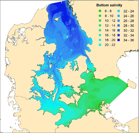
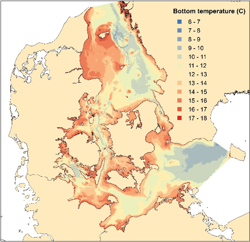
Annex figure 3. Predicted distributions of bottom salinity (left) and temperature (right) (August-October) from GAM model including month, depth, and position based on historical data (before 1970).
The spatial distribution of DObottom across the entire area highlighted that the area around the southern Little Belt, Flensburg Fjord and Aabenraa Fjord are most prone to oxygen depletion (Annex figure 4). For these areas neither severe oxygen depletion (<2 mg/l) nor oxygen depletion (<4 mg/l) was predicted anywhere for this first period, and low oxygen concentrations (<6 mg/l) was predicted for 3,229 km2. For the second period (1949-1969) severe oxygen depletion (<2 mg/l) was not predicted, whereas oxygen depletion (<4 mg/l) and low oxygen concentrations (<6 mg/l) were estimated to cover 584 km2 and 15,257 km2, respectively. Areas in Kiel Bay and Bay of Mecklenburg also showed relatively low oxygen concentrations, although above the oxygen depletion thresholds for the first period and with relatively small area below the oxygen depletion threshold for the second period. For both periods, the predicted bottom oxygen concentration remained above 4 mg/l for the Arkona Basin. Low oxygen concentrations (<6 mg/l) were found in Arkona Basin, Bay of Mecklenburg and Kiel Bay for the first period, whereas low oxygen concentrations were found in all areas for the second period. Following the approach of characterizing the first period (1900-1909) as reference condition and the last period (1949-1969) as target, threshold for the areal extent of oxygen depletion and low oxygen concentrations for HELCOM assessment units in the Danish Straits and Arkona Basin are proposed (Annex table 2).
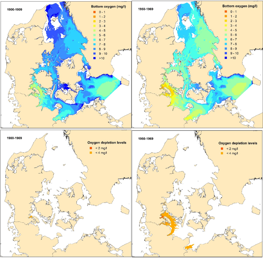
Annex figure 4. Predicted distribution of bottom oxygen concentrations (top row) and bottom oxygen concentrations below thresholds (bottom row) for the first period (left) and last period (right). Oxygen concentrations were predicted using the GAM model for oxygen. Oxygen conditions are not predicted for shallower depths than 10 m and cannot be predicted for the deepest part of the northern Kattegat, where predicted salinities are higher than the observations.
Annex table 2. Suggested reference conditions and target values for low oxygen concentration (<6 mg/l), oxygen depletion (<4 mg/l) and severe oxygen depletion (<2 mg/l) for the different HELCOM assessment units (excluding the coastal zone).
| Assessment Unit | Reference condition (1900-1909) | Target (1949-1969) | ||||
| Area < 2 mg/l | Area < 4 mg/l | Area < 6 mg/l | Area < 2 mg/l | Area < 4 mg/l | Area < 6 mg/l | |
| Arkona Basin | 0 km2 | 0 km2 | 2,782 km2 | 0 km2 | 0 km2 | 5,189 km2 |
| Bay of Mecklenburg | 0 km2 | 0 km2 | 206 km2 | 0 km2 | 228 km2 | 1,902 km2 |
| Belt Sea | 0 km2 | 0 km2 | 0 km2 | 0 km2 | 0 km2 | 1,043 km2 |
| Kattegat | 0 km2 | 0 km2 | 0 km2 | 0 km2 | 0 km2 | 5,257 km2 |
| Kiel Bay | 0 km2 | 0 km2 | 241 km2 | 0 km2 | 356 km2 | 1,696 km2 |
| The Sound | 0 km2 | 0 km2 | 0 km2 | 0 km2 | 0 km2 | 170 km2 |
| Entire area | 0 km2 | 0 km2 | 3,229 km2 | 0 km2 | 584 km2 | 15,257 km2 |
The status assessment for the last six years (2016-2021) in relation to the proposed target values show that none of the assessment units fulfils the ecological targets (Annex figure 5). Since oxygen depletion has severe and often lasting effects on e.g. bottom fauna, this is considered the ecological relevant indicator. However, other approaches for defining indicators and targets, using the overall method, may be suggested.
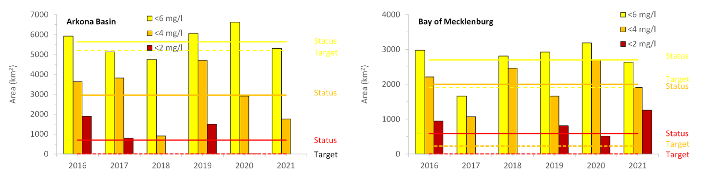
Annex figure 5. Areal extent of severe oxygen depletion (<2 mg/l), oxygen depletion (<4 mg/l) and low oxygen concentration (<6 mg/l) during the HOLAS 3 assessment period (2016-2021) for the different HELCOM assessment units calculated from the spatial interpolation model. The average for each of the three oxygen depletion indicators are compared with the proposed targets (Table 2).
Distribution of hypoxia in the past – deriving reference conditions and targets
For an indicator to become operational, targets need to be derived. For the oxygen debt indicator used for the Bornholm Basin and Gotland Basin, targets were derived based on estimated long-term trends in oxygen debt (HELCOM 2013). Using a change-point detection method, the period before ca. 1940 was considered relatively stable, which was followed by a drastic increase up to around 1980 after which the oxygen debt has remained stable. This trend corresponds well with the trends in nutrient inputs. Therefore, the period before 1940 was characterized as a reference condition with relatively little impact of eutrophication. Targets were derived by analysing the interannual variability of this period, using the upper 95% percentile of the annual oxygen debt distribution as target. This target corresponds to the situation around 1960.
Deriving reference conditions and targets for the entrance area to the Baltic Sea were developed using similar principles, i.e. assuming that the period before 1940 represented a reference condition and that the period around 1960 represented a target value. Since the development of hypoxia is more dynamic in this area and the number of historical oxygen profiles are fewer than for the central Baltic Sea, it is not possible to estimate trends of high temporal resolution of the areal extent of oxygen depletion.
For assessing the areal extent of oxygen depletion in the past, historical data prior to 1970 from the entrance area were obtained from the national marine monitoring database at Aarhus University. These data primarily originate from ICES, but there were also coastal data from national sources. Data from Limfjorden and Mariager Fjord were not included, since the mechanisms driving hypoxia in these two systems are different from the Danish Straits. Historical data from these two systems are too few for a separate analysis of oxygen conditions before 1970.
Only data from August-October and deeper than 10 m were analysed, totalling 1795 oxygen profiles of which 1434 were in the specific study area (Danish Straits and Arkona Basin) and 361 were from the western Bornholm Basin and the Skagerrak bordering the Kattegat (Annex figure 6). These latter profiles were included as bordering areas for the spatial interpolation (see below). The historical data represent conditions of severe oxygen depletion, mostly in the Little Belt, Flensburg Fjord and Aabenraa Fjord, and moderate oxygen depletion in Kiel Bay, Bay of Mecklenburg and north of Funen. Sporadic profiles with low oxygen concentrations are also spotted in the Arkona Basin. The earliest oxygen observations are from 1902, measured in Kiel Bay, Bay of Mecklenburg, Arkona Basin, and Kattegat. Most observations were from the 1950s and 1960s, but there were also a reasonable number of profiles in the 1930s and fewer in the 1900s and 1920s. No data were available for the 1910s, and only 7 profiles were available for the 1940s. Following the approach of using different periods to characterize reference and target conditions, the oldest data (1900-1909) were used to characterize the reference condition and data from the period 1950-1969 were used to characterize the target condition. The data from the intermediate period (1920-1939) were used to characterize a status between reference conditions and the target value (i.e. corresponding to a High-Good boundary). The reasons for not including data from 1920-1939 in the period representing reference conditions are that nutrient input from land has already risen from the early 1900 during these decades (Conley et al. 2007) and that time series of oxygen concentrations suggested decreasing conditions in all assessment units except Arkona Basin (Annex figure 7a). In fact, there is only one record of hypoxia in the first period (1900-1909) that was measured in the Little Belt (Belt Sea). The 7 profiles from the 1940s (Annex table 2) were included in this last period (1950-1969), as they are few and sampled in 1949. Hence, it is assumed that the first period (1900-1909) represents a situation with little eutrophication, the second period (1920-1939) represents a situation with a minor disturbance, and the last period (1949-1969) represents a target condition with acceptable deviation from the reference condition, corresponding to the approximate target year (1960) from HELCOM (2013), although spanning one decade to each side to ensure sufficient data for the analysis. The historical data also confirmed that the lowest oxygen concentrations are found at intermediate depths (20-40 m; Annex figure 7b), at salinities between 20 and 30 (Annex figure 7c) and temperatures around 10 °C (Annex figure 7d). These descriptive analyses suggest that it might be possible to predict oxygen concentrations from a combination of time, depth, salinity, and temperature.
Annex figure 6. Historical oxygen profiles (before 1970) from the entrance area to the Baltic Sea (Danish Straits and Arkona Basin). All profiles are based on discrete samples analysed by Winkler titration. The colour code shows the oxygen concentration of the deepest sample, which may not always represent the near-bottom water.
Annex table 2. Number of oxygen profiles (August-October) for the different assessment units and decades within the entrance area to the Baltic Sea. The number of discrete samples within each profile is highly variable.
| Assessment Unit | 1900-1909 | 1920-1929 | 1930-1939 | 1940-1949 | 1950-1959 | 1960-1969 |
| Arkona Basin | 20 | 15 | 46 | 2 | 59 | 329 |
| Bay of Mecklenburg | 3 | 1 | 10 | 2 | 63 | |
| Belt Sea | 13 | 4 | 78 | 5 | 261 | 82 |
| Kattegat | 17 | 1 | 51 | 3 | 135 | |
| Kiel Bay | 11 | 1 | 17 | 123 | 41 | |
| The Sound | 2 | 4 | 8 | 27 | ||
| Entire area | 64 | 24 | 206 | 7 | 456 | 677 |
Annex figure 7. Historical oxygen concentrations (before 1970) near the bottom versus time (a), depth (b), salinity (c), and temperature (d).
The areal distribution of hypoxia is estimated with the approach described above for the months from July to November, although only consistently for August-October where hypoxia is most widespread in the Danish Straits. Large inter-annual variations are observed in the spatial distribution of hypoxia (Figure 8), which is primarily governed by three factors (Conley et al. 2007): 1) nutrient inputs from land to the Danish Straits (stimulating algae production and thus, oxygen demand in bottom waters), 2) advective transports (supply of oxygen to bottom waters, primarily driven by wind conditions), and 3) temperature controlling the oxygen solubility of the Skagerrak surface water replenishing the bottom waters and stimulating respiratory processes. Hence, the effect of higher temperature is both a decrease in the supply of oxygen and an increase in microbial degradation rates and thereby oxygen consumption.
Most remarkable is that the southern part of Little Belt including Flensburg Fjord and Aabenraa Fjord exhibit severe oxygen depletion every year, and some years this patch of oxygen-deficient water stretches down into Kiel Bay (Annex figure 8). Bay of Mecklenburg including Lübeck Bay is another area prone to oxygen depletion, where oxygen concentrations in some years drop below 2 mg/l (severe depletion, hypoxia) and in some years oxygen concentrations are between 2 and 4 mg/l (moderate depletion). The water column in Little Belt, Kiel Bay and Bay of Mecklenburg is permanently stratified around 15 m, and oxygen is gradually depleted from the bottom water on a seasonal basis at a rate determined by temperature and organic matter input. However, oxygen-rich waters supplied through advective transports through the Great Belt can partly compensate the high oxygen demand, but this oxygen supply varies considerably among years. These areas operate as ‘dead ends’ for the bottom waters, due to the Darss sill and the contraction of the deeper parts in the northern Little Belt. This implies that considerable energy is required to ventilate these deeper waters and push the oxygen-deficient water either over the Darss sill, or through the narrow deeper channel of the northern Little Belt or by mixing with the surface layer. Another feature that contributes to oxygen depletion in the southern parts of Little Belt is the high primary production in Little Belt (Lyngsgaard et al. 2017) due to the intense mixing in the northern narrow part of Little Belt that brings nutrients into the photic zone. The resulting primary production then sediments out into the south floating bottom water and fuels a high oxygen demand in the southern part of the Little Belt.
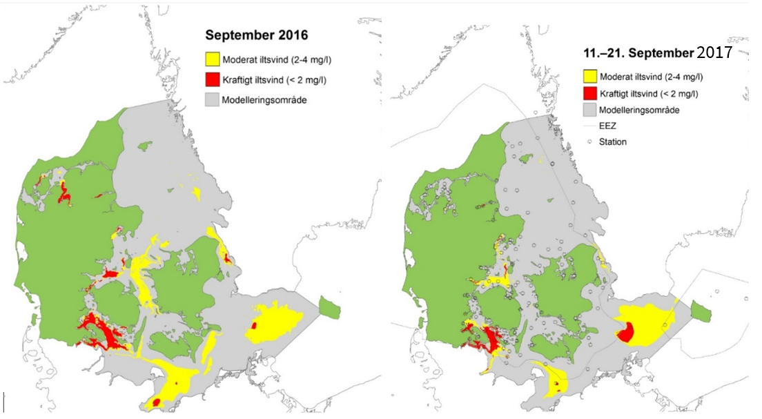
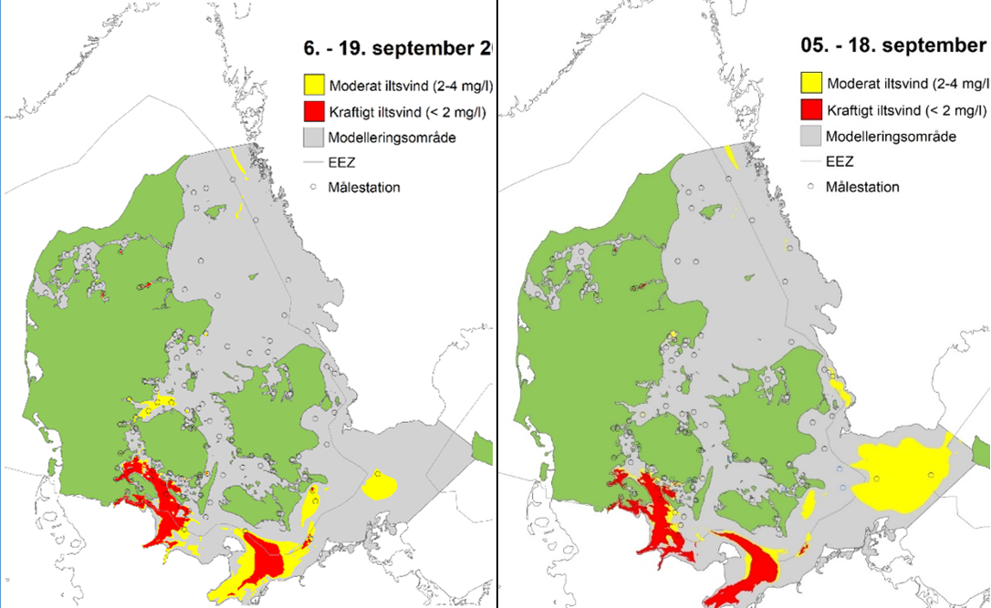
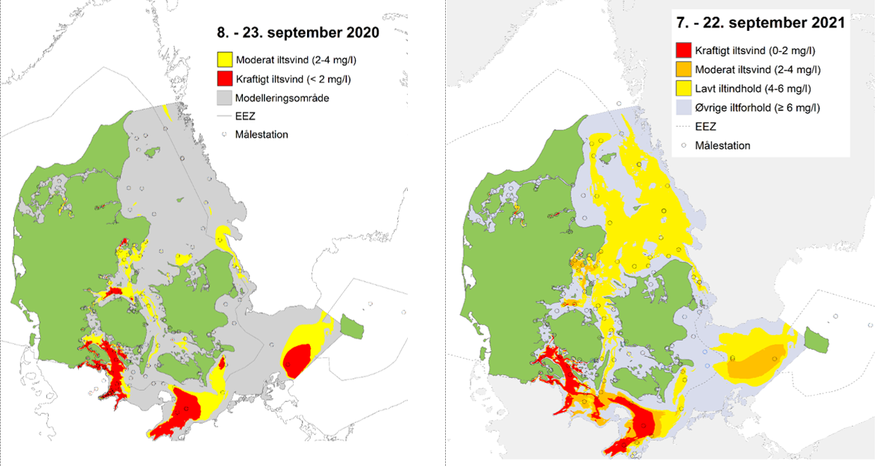
Annex figure 8. Areal distributions of severe oxygen depletion (<2 mg/l) and moderate oxygen depletion (2-4 mg/l) for the last six years (2016-2021) in September. The areal distribution of low oxygen depletion (<6 mg/l) is shown for 2021. Note that the colour coding is different for 2021. The areal distributions are estimated from oxygen profiles measured at the monitoring stations indicated by open circles. The model area is marked in grey.
The area north and south of Funen in the Belt Sea and Aarhus Bight also exhibit oxygen depletion at variable scale. Again, these three areas operate as terminal points for the bottom water inflows, although they are both more connected to the source of oxygen-rich waters from the northern Kattegat, implying that bottom water ventilation occurs more frequently, and the presence of hypoxia becomes more variable.
The Kattegat occasionally experience moderate oxygen depletion, and only severe oxygen depletion in exceptional years like 2002. Most of the Kattegat bottom waters are reasonably ventilated, although pockets of oxygen-depleted waters can occur north of Zeeland in some years. The Sound has a deep basin in its northern part, where stagnation can lead to oxygen depletion, mostly moderate oxygen depletion but in some years also severe oxygen depletion. The Drogden sill in the southern part of The Sound restricts the ventilation of the bottom waters.
The Arkona Basin receives denser bottom waters that flow over the two sills (Darss and Drogden) and form a thin bottom layer (typically 2-3 m). Depending on the frequency of these sill overflows and the ventilation of the thin bottom layer, hypoxia can develop in the Arkona Basin to a quite variable extent. In some years, oxygen depletion is absent in the Arkona Basin. The spatial location of the oxygen-depleted bottom waters depends on how the intrusions of denser water disperse in the Arkona Basin after crossing the sills.
The large variability in the areal extent is also visible when calculating the bottom areas with oxygen concentrations below the three thresholds for the different HELCOM assessment units and in total (Annex figure 9). The catastrophic 2002 stands out with an exceptionally large spread of hypoxia, covering an area almost twice as large as the second worst year. This year was remarkable, because oxygen-depleted waters spread to areas that are usually not exposed to oxygen depletion, such as the Kattegat and parts of the Belt Sea. However, the areal extent of this year was not exceptional for neither Bay of Mecklenburg nor Kiel Bay, where the areal extent of hypoxia often reaches its maximum given by the location of the permanent halocline. There is no apparent trend in the areal extent of oxygen depletion for any of the HELCOM assessment units across the last 33 years.
![]()
Annex figure 9. Time series of areal extent of severe oxygen depletion (<2 mg/l), oxygen depletion (<4 mg/l), and low oxygen concentration (<6 mg/l) in September for the different HELCOM assessment units and the entire area. The areas have been calculated from the spatial interpolation model.
It is recommended to use this approach for HOLAS 3 for assessing the oxygen conditions in the shallow waters of the entrance area to the Baltic Sea.
For the indicator to become operational, target values are needed. Historical data have been analysed to assess the extent of severe and moderate oxygen depletion in this area. However, due to the limited number of observations the same model approach could not be used for the historical extent of oxygen depletion. An alternative model approach has been developed, suggesting that in the early 1900s neither severe nor moderate oxygen depletion was present, but that low oxygen concentrations covered approximately 3,229 km2 of the offshore waters in an average year.
During the period 1949-1969, moderate oxygen depletion had expanded to 584 km2, severe oxygen depletion was still not present, whereas low oxygen concentrations were covering 15,257 km2. Following the approach used in HELCOM (2013), these areal extents (representing 1949-1969) are proposed as targets for the shallow water oxygen indicator. However, it is recommended to test the compliance between the spatial integration model used for the shallow water oxygen indicator and the model approach used for the historical data to ensure that the suggested target values apply for the proposed shallow water oxygen indicator.
The indicator presented here represents the maximal area affected by oxygen depletion in a given year and basin. The duration of oxygen depletion each year is not considered. These can be done for the assessment in recent years, but not for the historical values. Hence, it is not possible to compare the current values with a threshold defined from historical data, but it is possible to monitor the development over time in both area and duration of oxygen depletion.
Annex B: Shallow water oxygen indicator approach for the Gulf of Bothnia
Reference levels
Data on near bottom water oxygen in late summer (July- October) before 1940 is scarce and only available for few stations in the Gulf of Bothnia. The time interval used for setting reference values (phase before notable eutrophication induced oxygen decline) was selected based on break-point detection of oxygen debt data calculated in HELCOM Targrev project (Rodionov 2004). Based on the detected breakpoints, data before 1968 was used for Bothnian Sea and data before 1979 for Bothnian Bay. For the Quark, the breakpoint detected for Bothnian Sea (1968) was used. For more information on the break-point detection for the Gulf of Bothnia, see document State & Conservation 5E-2017 3-2.
The proposed reference levels were primarily set based on data from the reference period. In the Bothnian Bay, the reference values were similar between stations, ranging between 11.2-12.0 mg L-1 for all stations except for F13 near the Quark-Bothnian Bay border, where the value was 10.7 mg L-1 (Annex table3). Using the acceptable deviation of 25 %, the tentative thresholds ranged from 8,1- 9,0 mg L-1 with mean of 8.8 mg L-1. In test assessment the status in 2016-2021 is high for all stations. The number of available data from the reference period is quite low for all stations, but the similarity between the station reference values gives support to the results.
Annex table 3. Proposed reference values and thresholds (G/M boundaries), and a test status assessment of saturation adjusted near-bottom oxygen for the stations in the Bothnian Bay open-sea assessment unit (SEA-017). The reference value and the threshold for the assessment unit are the means of the station specific values.
| Site | N reference period
(1905-1979) |
Tentative reference value
(mgL-1) |
Tentative G/M boundary | ES 2016-2021 (mg L-1) | EQR
2016-2021 |
Status class |
| BO3 | 11 | 11,2 | 8,4 | 11,2 | 0,99 | High |
| CV | 5 | 12,0 | 9,0 | 11,8 | 0,98 | High |
| CVI | 6 | 11,7 | 8,8 | 12,0 | 1,00 | High |
| F13 | 17 | 10,7 | 8,1 | 9,8 | 0,91 | High |
| F2 | 8 | 12,0 | 9,0 | 11,7 | 0,98 | High |
| F3 / A5 | 10 | 12,0 | 9,0 | 12,1 | 1,00 | High |
| F9 | 13 | 11,9 | 8,9 | 11,7 | 0,98 | High |
| RR3 | 8 | 12,0 | 9,0 | 12,0 | 1,00 | High |
| RR6 | 10 | 11,9 | 8,9 | 11,8 | 0,99 | High |
| RR7 | 10 | 12,0 | 9,0 | 11,5 | 0,96 | High |
| SEA-017 | 11,7 | 8,8 |
In the Bothnian Sea and the Quark, there is a clear decreasing tendency in the near-bottom oxygen concentrations. The average oxygen concentrations in the reference period (1906- 1969) ranged from 7.9- 11.6 mg L-1 (Annex table 4, Annex table 5). Data from the reference period is lacking or very sparse for most of the monitoring stations. The reference values were therefore estimated also by extrapolating linear trends in oxygen concentrations: Median slope of site-specific linear trends (1940-2021) was used to extrapolate oxygen concentrations in 1940 from the present oxygen concentrations (mean of 2011-2020) (Annex table 4, Annex table 5). The proposed thresholds were selected followingly: If the number of samples from the reference period was ≥10, the median from the reference period was chosen, and otherwise the linearly extrapolated threshold was chosen. The resulting reference values ranged from 8.6 – 11.8 mg L-1 for Bothnian Sea and from 9.9- 11.4 mg L-1 for the Quark. Using 25% acceptable deviation, the tentative thresholds ranged from 6.4- 8.9 mg L-1 (mean 7.7 mg L-1) for the Bothnian Sea and from 7.4- 8.5 mg L-1 (mean 8.1 mg L-1) for the Quark.
Annex table 4. Reference values and thresholds (G/M boundaries), and test status assessment of saturation adjusted near-bottom oxygen for the stations in the Bothnian Sea open-sea assessment unit (SEA-015), based on data from the reference period (before 1969) and on extrapolation of the negative trend in oxygen concentrations from 1940-2021 using median slope (-0.025) of site-specific trends for the change in saturation adjusted oxygen. The reference value and the threshold for the assessment unit are the means of the station specific values.
| Site | N reference period (1906-1968) | Reference value based on median 1906-1968 (mgL-1) | Reference value based on linear models (mgL-1) | ES (2016-2021) (mgL-1) | Tentative reference value | Tentative G/M boundary | EQR | Class | Reference value setting method |
| C3 | 8,6 | 7,1 | 8,6 | 6,4 | 0,82 | Good | linear extrapolation | ||
| F26 | 12 | 9,8 | 9,4 | 7,5 | 9,8 | 7,4 | 0,77 | Good | reference period median |
| F33 | 11 | 11,5 | 11,9 | 10 | 11,5 | 8,6 | 0,87 | High | reference period median |
| MS3 | 2 | 9,4 | 9,5 | 7,6 | 9,5 | 7,1 | 0,81 | Good | linear extrapolation |
| MS4 / C14 | 1 | 7,9 | 9,1 | 7 | 9,1 | 6,8 | 0,78 | Good | linear extrapolation |
| MS6 | 3 | 7,6 | 11 | 9,1 | 11 | 8,2 | 0,83 | Good | linear extrapolation |
| MS8 | 2 | 8 | 8,8 | 7,1 | 8,8 | 6,6 | 0,81 | Good | linear extrapolation |
| MS9 | 1 | 10,8 | 10,7 | 8,9 | 10,7 | 8 | 0,83 | Good | linear extrapolation |
| SR3 | 2 | 10,8 | 11,5 | 9,7 | 11,5 | 8,6 | 0,84 | Good | linear extrapolation |
| SR5 | 15 | 10,9 | 10,6 | 9,2 | 10,9 | 8,2 | 0,85 | Good | reference period median |
| SR7 | 11,8 | 10 | 11,8 | 8,9 | 0,84 | Good | linear extrapolation | ||
| SR8 | 14 | 11,4 | 12 | 10,2 | 11,4 | 8,6 | 0,89 | High | reference period median |
| US3 | 1 | 9,3 | 9,1 | 7,2 | 9,1 | 6,8 | 0,8 | Good | linear extrapolation |
| US5B | 9 | 7,5 | 9 | 6,8 | 0,83 | Good | linear extrapolation | ||
| US6B | 10,3 | 8,5 | 10,3 | 7,7 | 0,82 | Good | linear extrapolation | ||
| US7 | 3 | 10,9 | 11,1 | 9,3 | 11,1 | 8,4 | 0,83 | Good | linear extrapolation |
| SEA-015 | 10,3 | 7,7 |
Annex table 5. Reference values and thresholds (G/M boundaries), and test status assessment of saturation adjusted near-bottom oxygen for the stations in the Quark open-sea assessment unit (SEA-016), based on data from the reference period (before 1969) and on extrapolation of the negative trend in oxygen concentrations from 1940-2021 using median slope (-0.025 ) of site-specific trends for the change in saturation adjusted oxygen. The reference value and the threshold for the assessment unit are the means of the station specific values.
| Site | N reference period (1906-1968) | Reference value based on median 1906-1968 (mgL-1) | Reference value based on linear models (mgL-1) | ES (2016-2021) (mgL-1) | Tentative reference value | Tentative G/M boundary | EQR | Class | Reference value setting method |
| F15 | 2 | 11,6 | 11,3 | 9,5 | 11,3 | 8,5 | 0,84 | Good | linear extrapolation |
| F16 | 6 | 10,6 | 11,4 | 9,2 | 11,4 | 8,5 | 0,81 | Good | linear extrapolation |
| F18 | 5 | 10,4 | 9,9 | 7,9 | 9,9 | 7,4 | 0,8 | Good | linear extrapolation |
| SEA-016 | 10,9 | 8,1 |
The indicator estimates the temporal change in near-bottom oxygen concentration in July – October, when the oxygen concentrations are lowest, from the reference period to the assessment period. In order to exclude the effect of increasing temperature on oxygen solubility from the observed negative trends in oxygen concentration, the oxygen concentrations were first transformed to oxygen saturation as described in HELCOM COMBINE manual, and the oxygen saturation values where then calculated back to “saturation corrected oxygen concentrations” using oxygen solubility at site specific average near-bottom temperatures and salinities. The effect of saturation correction was small, but consistent (Annex figure 10).
Annex figure 10. Temporal development of near bottom oxygen in example stations from the Bothnian Sea and the Bothnian Bay. Measured oxygen concentrations are marked on dark and saturation corrected concentrations on green. The lines show the linear models.