 Seafloor litter
2 Relevance of the indicator
Once litter is introduced in the marine environment it can be transported long distances by water currents and accumulate on the seafloor far away from its original source. Recent reviews indicate that the density of macro-scale (>2 cm) litter items is higher on the seafloor than floating on the sea surface (Galgani et al., 2015), suggesting that a large part of the total amount of litter in the marine environment is deposited on the seafloor. The negative impacts of litter that is deposited on the seafloor are wide ranging including death of marine organisms by entanglement and lack of oxygen, ingestion, contamination, smothering and other damage to habitats, and can also have socioeconomic impacts, and may pose navigational hazards.
2.1 Ecological relevance
Litter on the seafloor can cause anoxia to the underlying sediments, which alters biogeochemistry and benthic community structure (Goldber, 1994). Furthermore, litter (such as glass bottles, tin cans) may provide substrata for the attachment of sessile biota in sedimentary environments and increase local diversity (Mordecai et al., 2011; Moret-Ferguson et al., 2010; Pace et al., 2007). This may replace existing species and leads to non-natural alterations of faunal community composition (Bergmann & Klages, 2012). Heavy plastic items may be colonized by bacteria or loaded with sediments and sink to the seafloor (Thompson, 2006; Ye & Andrady, 1991) where they can persist for centuries (Derraik, 2002), or may be ingested by organisms. Litter containing hazardous substances can act as source to these, and thereby contribute to pollution effects in the ecosystem. The monitoring of seafloor litter is required to close the loop of marine litter monitoring in the aquatic environment.
2.2 Policy relevance
At this moment in time, marine litter is perceived as an important problem. The historic agreement at the resumed Fifth Session of the United Nations Environment Assembly (UNEA 5-2) in March 2022 to develop an international legally binding agreement to end plastic pollution by 2024 is a clear example of such global commitment. HELCOM is committed to support the development of the global instrument, as stated in a voluntary commitment on the matter at the UN Ocean Conference held in Lisbon in June 2022. In alignment with such commitment, the updated Baltic Sea Action Plan contains, for the first time, a dedicated section on marine litter including both ecological and managerial objectives to achieve. The fulfilment of these objectives will count with the revised Regional Action Plan on Marine Litter, adopted in the 2021 Ministerial Meeting as HELCOM Recommendation 42-43/3, as its instrumental tool containing almost thirty regional actions addressing sea-based and land-based sources of marine litter (HELCOM, 2021a). Moreover, in its preamble, the Action Plan states HELCOM ambitions towards development of additional core indicators and associated definition of GES and improved coordinated monitoring programmes. Such work is to be conducted considering outcomes of the related work under the EU MSFD and involving close coordination with the EU TG Litter, as well as with similar work of the Russian Federation.
In that sense, recommendations for sampling seafloor litter (specifying shallow and deeper waters) are derived from the MSFD GES Technical Group on Marine Litter (JRC, 2013) to contribute to the monitoring of litter in the marine environment according to the MSFD requirements. Seabed litter is also a common indicator of the OSPAR area, as detailed in the Second Regional Action Plan for Prevention and Management of Marine Litter in the North-East Atlantic (OSPAR, 2022).
Table 2. Policy relevance of this specific HELCOM indicator.
| Baltic Sea Action Plan (BSAP) | Marine Strategy Framework Directive (MSFD) | |
| Fundamental link | Ecological objective: No harm to marine life from litter.
Management objectives: (i) Prevent generation of waste and its input to the sea, including microplastics; (ii) Significantly reduce amounts of litter on shorelines and in the sea. |
Descriptor 10 Properties and quantities of marine litter do not cause harm to the coastal and marine environment.
|
| Complementary link | Management objectives: (i) Minimize the input of nutrients, hazardous substances and litter from sea-based activities; (ii) Safe maritime traffic without accidental pollution | Descriptor 10 Properties and quantities of marine litter do not cause harm to the coastal and marine environment.
|
| Other relevant legislation | UN Sustainable Development Goal 14 (Conserve and sustainably use the oceans, seas and marine resources for sustainable development) is most clearly relevant, though SDG 12 (Ensure sustainable consumption and production patterns) and 13 (Take urgent action to combat climate change and its impacts) also have relevance. | |
2.3 Relevance for other assessments
The indicator assesses the 2021 Baltic Sea Action Plan’s (BSAP) (HELCOM 2021) Hazardous substances and litter’s segment ecological objective of no harm to marine life from litter. It also assesses the management objectives to prevent generation of waste and its input to the sea, including microplastics, and significantly reduce amounts of litter on shorelines and in the sea. The indicator is relevant to the following specific BSAP action:
- HL32 Agree on core indicators and harmonized monitoring methods to evaluate quantities, composition, distribution, and sources (including riverine input), of marine litter, including microlitter, by 2022, where applicable and for the rest no later than 2026. Work should be done in close coordination with work undertaken by Contracting Parties in other relevant fora, such as the Technical Group on marine litter under the Marine Strategy Framework Directive.
The indicator further supports the implementation of the HELCOM Recommendation 42-43/3 on the Regional Action Plan on Marine Litter, in particular action RL2 on the evaluation of top findings according to the knowledge available and recommendation of environmentally sound alternatives to phase out top plastic and rubber litter items.
The results of the indicator support an overall evaluation of pollution in the Baltic Sea.
Potential relevance for indicators for different types of hazardous substances, like flame retardants, used as plastic additives.
In addition, the indicator addresses descriptor 10 “Properties and quantities of marine litter do not cause harm to the coastal and marine environment” of the EU MSFD for determining good environmental status (European Commission 2008), and in particular criteria 1 and 2 of the Commission Decision on GES criteria (2017), “The composition, amount and spatial distribution of litter on the coastline, in the surface layer of the water column, and on the seabed, are at levels that do not cause harm to the coastal and marine environment”, and “The composition, amount, and spatial distribution of micro-litter on the coastline, in the surface layer of the water column, and in seabed sediment, are at levels that do not cause harm to the coastal and marine environment”, respectively. The complementary link to criteria 2 is due to the fragmentation of macrolitter to microlitter.
3 Threshold values
The evaluation is based on a trend not significantly >0 (preliminary).
3.1 Setting the threshold value(s)
The threshold was set as no significant increase over the observed time period in the monitored part of the Baltic Sea. The threshold is preliminary and for use only until further guidance is available.
4 Results and discussion
The temporal development in mass and number of litter items caught per km2 and probability of catching litter in a haul in the surveyed area can be seen in figures 1, 2 and 3, respectively. By far the most numerous litter item in terms of number and probability was plastic, followed by natural litter (Table 3). The trend estimated for the different litter types differ depending on whether the early (poorly sampled) years are included as well as between densities measured by numbers and weight (Table 4). Among the plastic items counted, SUP (as defined in Table 8) accounted for 36% (32% by weight). As the changes in early years may be a result of differences in sample coverage and effort, the trends are examined from 2015 onwards. The spatial distribution of the assessed litter types can be seen in figure 4. The large differences in the distribution as measured by weight and numbers/probability of catch is likely due to differences in sample coverage and effort as all years are included in the estimation of the distribution of litter. Annual estimates from model 1 (please see chapter 9.2.3 for further information) are given in Table 5.
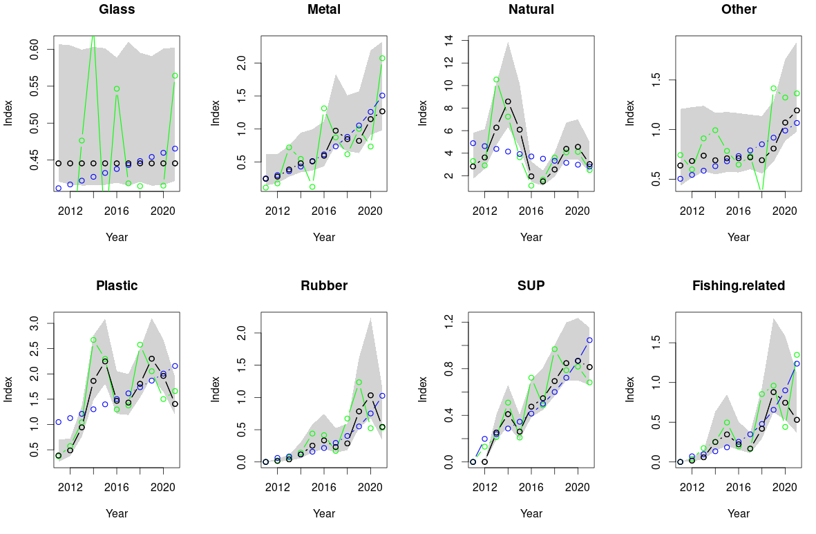
Figure 1. Temporal development in kg litter/km2 as estimated by models 1 (black, grey is 95% confidence interval of the estimate), 2 (green) and 3 (blue). Top row from left to right: glass, metal, natural, other. Bottom row from left to right: plastic, rubber, SUP, fisheries related plastic. Note difference in scale of the y-axis.
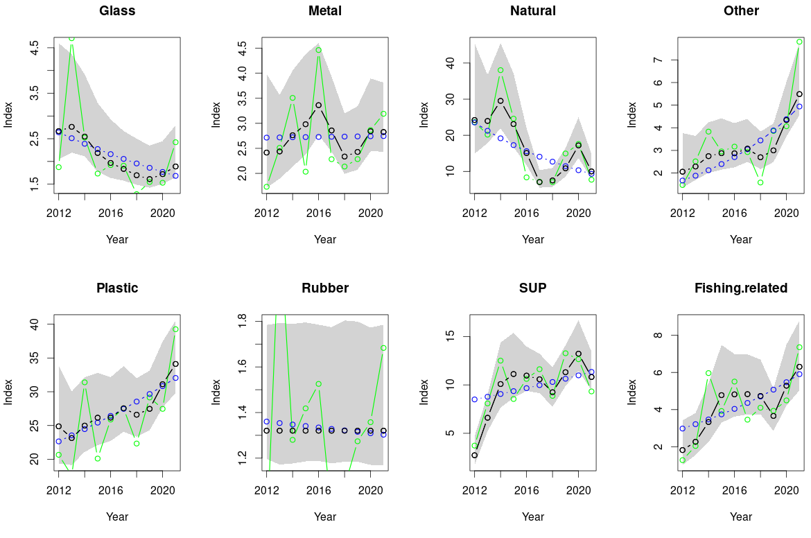
Figure 2. Temporal development in number of litter items/km2 as estimated by models 1 (black, grey is 95% confidence interval of the estimate), 2 (green) and 3 (blue). Top row from left to right: glass, metal, natural, other. Bottom row from left to right: plastic, rubber, SUP, fisheries related plastic. Note difference in scale of the y-axis.
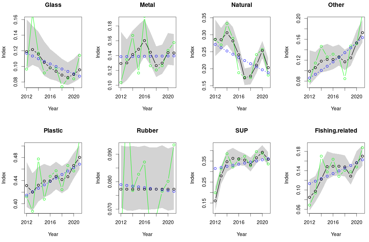
Figure 3. Temporal development in probability of catching litter as estimated by models 1 (black, grey is 95% confidence interval of the estimate), 2 (green) and 3 (blue). Top row from left to right: glass, metal, natural, other. Bottom row from left to right: plastic, rubber, SUP, fisheries related plastic. Note difference in scale of the y-axis.
Table 3. Average weight and number of litter items per km2 and probability of non-zero catch across all years. Note that the number of hauls analysed for weight and number differs, and hence the numbers are not directly comparable.
| Average weight kg/km2 | Average Probability/haul | Average Number/km2 | |
| Glass | 0.45 | 0.101 | 2.09 |
| Metal | 0.73 | 0.140 | 2.72 |
| Natural | 4.25 | 0.242 | 16.86 |
| Other | 0.80 | 0.126 | 3.15 |
| Plastic | 1.59 | 0.444 | 27.22 |
| Rubber | 0.36 | 0.077 | 1.32 |
| SUP | 0.52 | 0.331 | 9.67 |
| Fishing related | 0.36 | 0.135 | 4.181 |
| Total | 1.13 | 8.40 |
Table 4. Trend and significance level of trend in weight and number of litter items per km2. Trends in probability of non-zero catch are identical to trends in numbers. Effects greater than 0 indicate increase and effects smaller than 0 indicate decrease. Values in bold indicate significant trends.
| Weight | Number | |||||||
| All years | 2015 onwards | All years | 2015 onwards | |||||
| Litter type | effect | P | effect | P | effect | P | effect | P |
| Glass | 0.012 | 0.563 | 0.0234 | 0.451 | -0.05 | 0.0438 | 0.0169 | 0.642 |
| Metal | 0.179 | <0.0001 | -0.015 | 0.558 | 0.0013 | 0.952 | -0.0217 | 0.476 |
| Natural | -0.550 | 0.007 | -0.0654 | 0.0177 | -0.103 | <0.0001 | -0.0439 | 0.146 |
| Other | 0.075 | 0.00454 | 0.153 | <0.0001 | 0.1206 | <0.0001 | 0.1532 | <0.0001 |
| Plastic | 0.072 | <0.0001 | 0.0935 | <0.0001 | 0.0386 | 0.0021 | 0.0432 | 0.0131 |
| Rubber | 0.311 | <0.0001 | 0.039 | 0.272 | -0.0048 | 0.868 | 0.00947 | 0.816 |
| SUP | 0.185 | <0.0001 | -0.015 | 0.36 | 0.0321 | 0.01876 | -0.00179 | 0.924 |
| Fisheries related | 0.317 | <0.0001 | 0.102 | 0.0016 | 0.0761 | 0.00158 | 0.04431 | 0.169 |
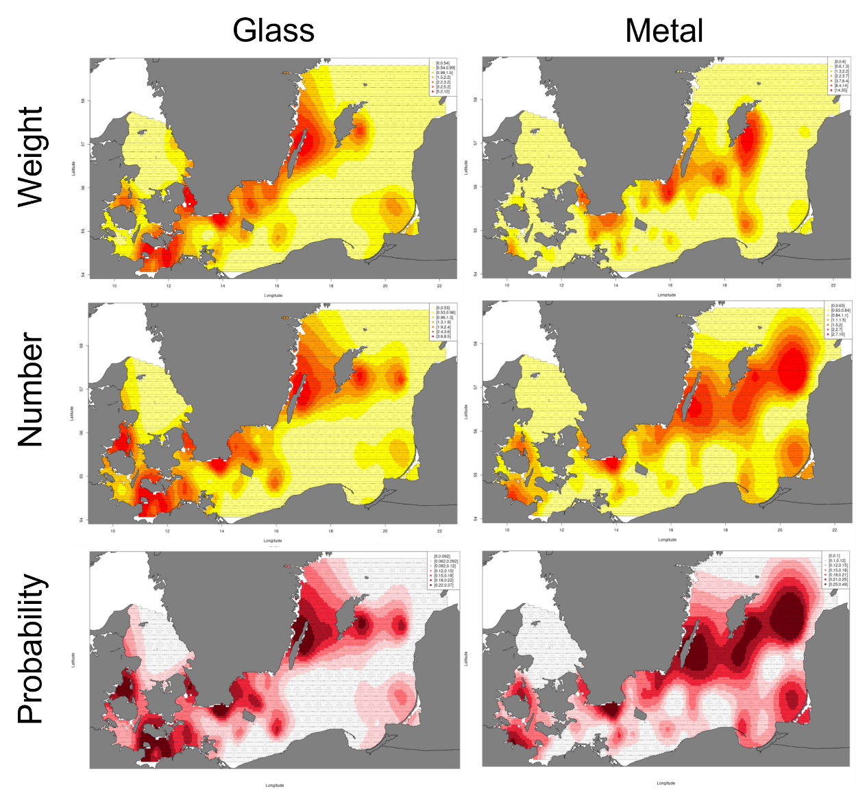 Figure 4a. Distribution of different litter types in weight, number and probability of catching litter. Colouring reflects amount relative to the mean, yellow/white is low amounts, red/dark red is high amounts. Note the limited sampling in deeper areas, see figure 3, and that the areas presented are not directly compatible with the standard HELCOM Assessment Units.
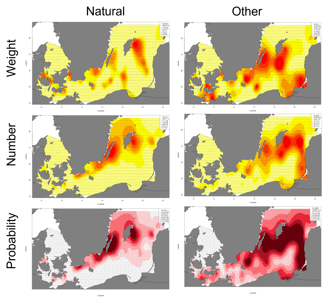 Figure 4b. Distribution of different litter types in weight, number and probability of catching litter. Colouring reflects amount relative to the mean, yellow/white is low amounts, red/dark red is high amounts. Note the limited sampling in deeper areas, see figure 3, and that the areas presented are not directly compatible with the standard HELCOM Assessment Units.
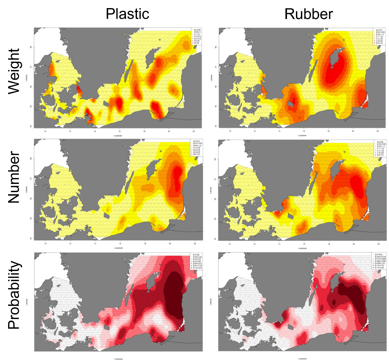 Figure 4c. Distribution of different litter types in weight, number and probability of catching litter. Colouring reflects amount relative to the mean, yellow/white is low amounts, red/dark red is high amounts. Note the limited sampling in deeper areas, see figure 3, and that the areas presented are not directly compatible with the standard HELCOM Assessment Units.
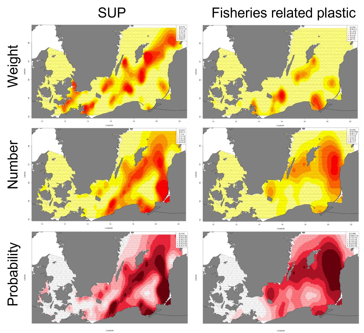
Figure 4d. Distribution of different litter types in weight, number and probability of catching litter. Colouring reflects amount relative to the mean, yellow/white is low amounts, red/dark red is high amounts. Note the limited sampling in deeper areas, see figure 3, and that the areas presented are not directly compatible with the standard HELCOM Assessment Units.
4.1 Discussion
When litter density was measured in weight, the categories “other”, plastic and fisheries related litter increased significantly in the period from 2015 to 2021 whereas when density was measured in numbers, only the categories “other” and plastic litter increased significantly (see Table 5 below). Hence, the categories “other” and plastic litter failed the preliminary threshold of no significant increase from 2015 to 2021 in both weight, numbers and probability of catching litter. Fisheries related litter passed the threshold when measured in numbers per km2 but not when measured in weight per km2. The categories glass, metal, natural, rubber and SUP showed no significant increase in weight and numbers per km2 and hence passed the preliminary threshold of no significant increase.
Table 5. Evaluation of the preliminary threshold of no significant increase from 2015 to 2021.
| HELCOM Assessment unit name (and ID) | Threshold value achieved/failed | Distinct trend between current and previous evaluation | Description of outcomes, if pertinent |
| Baltic Sea | Achieved for glass, metal, natural litter, fisheries related litter (numbers only) rubber and SUP | Stable/decreasing | Indicator evaluation failed to achieve the threshold value for some litter categories. Long degradation time for most litter types. |
| Failed for plastic, fisheries related (weight only) and other litter. | Increasing |
5 Confidence
Confidence in the applied threshold value is high, given that the choice is based on a policy decision. The data coverage is good within the surveyed area and period, but the amount of litter observed varies greatly between trawl hauls and even after the addition of a state of the art-statistical model to account for this variability, the coefficient of variation (CV) around the annual estimates of litter on the seafloor remain high.
6 Drivers, Activities, and Pressures
As the deep seafloor is thought to constitute a sink/accumulation area also for marine litter, most sources for marine litter can probably contribute to litter on the seafloor. Recent reviews of the amount and composition of litter on the seafloor show that items associated with maritime activities (e.g., fishing, shipping) dominate in some areas, but that items from land-based sources also commonly occur (Galgani et al., 2010; Galgani et al., 2015; Pham et al., 2014). In addition to that, seafloor litter can affect the ecosystem and its integrity, it should also be recognised that litter in the sea can have a socio-economic impact on human activities related to the sea, e.g., costs for damage to or loss of fishing gear, obstruction of motors, beach cleanups subsequently washed ashore and potential effects on tourism and recreation (Newman et al., 2015).
Fishing gear that has been lost, so called ghost nets, are a very special type of anthropogenic litter on the seafloor. Ghost nets are known to continue fishing and can be considered as posing an especially large risk to the environment compared to other types of litter. Static and bottom trawling fishing gear are known to be frequently lost and/or discarded. Studies have estimated the total catch of cod by ghost nets to 3-906 tonnes during a 28 month study period, amounting to 0.01-3.2% of the total weight of reported and landed cod catch from the same area and time period (Brown et al., 2005).
The types of gear lost and the reasons for the gear being lost are believed to differ regionally in the Baltic Sea, however comprehensive statistics are currently not available. In 2011, WWF Poland together with fishermen, scientists and divers conducted a pilot project financed by Baltic Sea 2020, with a view to work out the methodology for net removal and carry out activities to clean the Polish territorial waters from ghost nets. As a result, 6 tonnes of ghost nets were retrieved from the Baltic during 24 days of actions at sea – from sea bottom and two ship wrecks. In 2014, a ghost net project was conducted by the Ozeaneum Stralsund, archeomare e.V., Drosos foundation and the WWF Germany on Rügen. In that project divers removed around 4 tonnes of ghost nets from 2 wrecks.
New data on the occurrence of derelict fishing gear (DFG) in the Baltic were collected through MARELITT Baltic, an EU-supported project involving partners from Estonia, Germany, Poland and Sweden. One of the aims of the project was to develop cost-efficient methods for mapping the occurrence of DFG, and to develop cost-efficient and environmentally sound methods for collecting DFG. The project ran for the period 2016-2019 (MARELITT, 2019).
7 Climate change and other factors
Climate change does not impact seafloor litter except through possible changes in transport of litter by e.g., wind, rivers or currents.
8 Conclusions
Litter in the categories “other”, plastic and fisheries related litter failed the threshold of no increase but only “other” and plastic litter failed the threshold of no increase in both weight, numbers and probability of catching litter. Fisheries related litter passed the threshold when measured in numbers per km2 but not when measured in weight per km2. The categories glass, metal, natural, rubber and SUP showed no significant increase in weight and numbers per km2 and hence passed the preliminary threshold of no significant increase. The confidence in the trend estimate from the model is high, but the high variability in the data decreases the confidence in the annual values.
In addition, data collected prior to 2015/2018 are considered less reliable because even though the sampling of litter in the Baltic Sea International Trawl survey commenced in 2011, the manual describing the categories and sample codes was not fully standardised until 2015 and a common description of how to conduct the sampling was not available until 2018.
8.1 Future work or improvements needed
Further improvements to the analysis could include monitoring of the amount of litter in categories more closely related to ingestion, entanglement and contaminants. Further, the issue of the source of litter items should be investigated in order to suggest appropriate management measures and likely impacts of these on the indicator.
9 Methodology
9.1 Scale of assessment
The indicator is assessed at HELCOM level 1 (entire Baltic Sea), with the caveat that it is based on ICES coordinated trawl surveys and that there is no sampling north of the Gotland basins, on rough grounds, in coastal areas, or on grounds with dumped munition (HELCOM Monitoring and Assessment Strategy Annex 4). There are no plans to expand the coverage of the currently used surveys.
9.2 Methodology applied
Benthic trawls such as the ones used in the Baltic Sea International Trawl Survey (figure 5) are designed to capture demersal fish species on the seafloor over a range of different seabed types that can be trawled. The trawl interacts with the seafloor in several places, hence, smaller litter and heavy litter can be carried into the water, and subsequently this litter enters the trawl where it may either pass through the mess or be retained. In the Baltic, the TV3 trawl is used in a small and a large version which are effectively scaled versions of the same gear. The widest part of the trawl is between the trawl doors (figure 5). The ground gear consists of a series of 10 cm wide rubber discs that roll over the bottom, creating turbulence that may cause the trawl to pass over or lift litter into the net. The turbulence differs between soft and harder bottom types. The initial part of the net has large meshes (8-12 cm) and only the very final part of the net has small meshes (2 cm). Hence, smaller litter can be carried through the meshes of the initial part of the trawl and thus do not occur among the items brought onboard the vessel whereas larger litter once entering the trawl mouth will be retained. The water current will also affect how much of the litter is retained as a strong current may affect the amount of water passing through the trawl and hence the amount of floating litter encountered. The trawl is therefore likely to under-represent the number of small and heavy items as these pass through the meshes of the net or do not even enter the trawl. As bottom trawls of different types are dragged at different distances above the sediment it is still difficult to predict how much of the actual litter on the bottom is caught by the trawl as this is not studied. Further, trawl surveys cover only sandy or muddy/clay areas and hence do not represent rocky substrates which may retain different amounts of litter. Finally, there are some concerns over the quality of the data submitted as the sampling guidelines and quality control have undergone continued development from the onset of litter sampling to today. The latest sampling protocol can be found at ICES (2022).
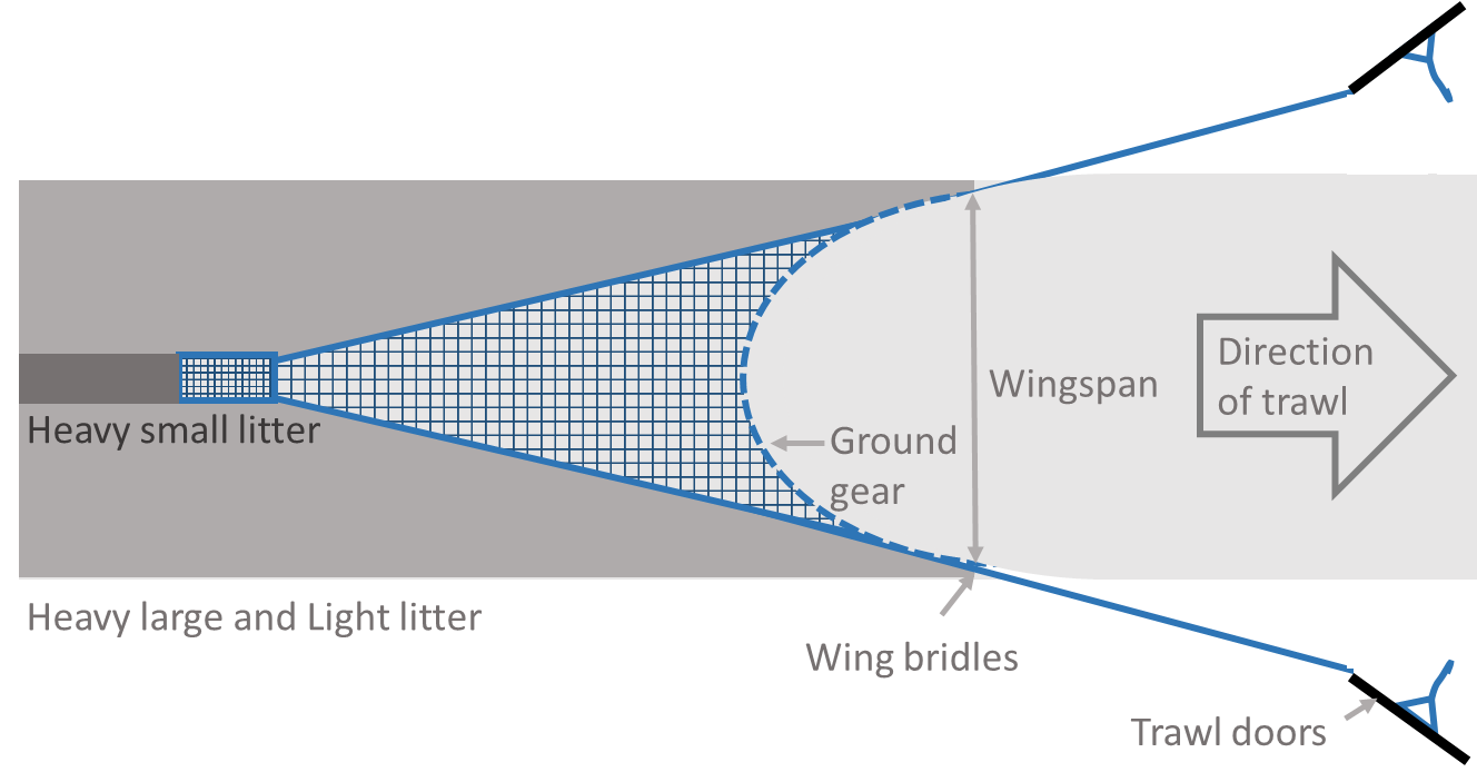
Figure 5. The active region of a benthic trawl net for light and heavy litter. Text indicates the types of litter not retained in each part of the trawl path. All litter except very small items are retained in the darkest grey part of the trawl path.
9.2.1 Data preparation
Data for use in the analysis were extracted from the ICES website (https://datras.ices.dk/Data_products/Download/Download_Data_public.aspx). The methods outlined below are similar to methods used by OSPAR in the assessment of marine litter.
The sampling of litter in the Baltic Sea International Trawl survey commenced in 2011 but a description of the categories and sample codes was not fully standardised until 2015. A common description of how to sample litter did not appear until 2018. In the early years, some countries reported numbers while others reported weight. Further, the categories used initially were coarser than those currently used. As a result, data collected prior to 2015/2018 are considered less reliable. The locations sampled annually in the survey are shown in figure 6. There are minor variations in survey location within the surveyed area between years. The north-eastern Baltic is not covered by the available data. This area must therefore be monitored using other data if an evaluation of the development over time in litter density is to be conducted.
Figure 6. Sampling locations (red) and depth (shades of blue). Note that deep and the north and north-eastern part of the Baltic is not sampled. Please note that the depth map is not indicative of HELCOM agreed borders.
Litter data are recorded in the database by Denmark, Estonia, Germany, Lithuania, Latvia, Poland, Russia and Sweden. The years sampled for litter weight and litter number varies between countries (Tables 6 and 7). From 2016 onwards, the proportion of hauls recording both litter weight and numbers has been above 85% (Figure 7).
Table 6. Number of hauls sampled by country for weight of litter.
| Year | Denmark | Estonia | Germany | Latvia | Lithuania | Poland | Russia | Sweden |
| 2011 | 194 | 0 | 0 | 0 | 0 | 0 | 0 | 0 |
| 2012 | 203 | 0 | 51 | 0 | 0 | 0 | 0 | 80 |
| 2013 | 192 | 0 | 104 | 0 | 0 | 0 | 0 | 74 |
| 2014 | 146 | 0 | 115 | 0 | 0 | 0 | 0 | 70 |
| 2015 | 169 | 9 | 107 | 14 | 2 | 31 | 0 | 78 |
| 2016 | 95 | 10 | 116 | 41 | 10 | 95 | 0 | 76 |
| 2017 | 91 | 10 | 108 | 49 | 11 | 136 | 0 | 78 |
| 2018 | 205 | 10 | 111 | 56 | 9 | 118 | 16 | 63 |
| 2019 | 157 | 6 | 98 | 44 | 12 | 127 | 0 | 68 |
| 2020 | 222 | 8 | 108 | 37 | 12 | 106 | 0 | 68 |
| 2021 | 235 | 7 | 103 | 43 | 0 | 119 | 14 | 72 |
Table 7. Number of hauls sampled by country for number of litter items.
| Denmark | Estonia | Germany | Latvia | Lithuania | Poland | Russia | Sweden | |
| 2012 | 52 | 0 | 51 | 0 | 0 | 0 | 0 | 60 |
| 2013 | 0 | 0 | 104 | 0 | 0 | 0 | 0 | 64 |
| 2014 | 0 | 0 | 115 | 0 | 0 | 0 | 0 | 57 |
| 2015 | 15 | 9 | 107 | 14 | 3 | 31 | 0 | 57 |
| 2016 | 95 | 10 | 116 | 41 | 10 | 95 | 0 | 57 |
| 2017 | 91 | 10 | 108 | 49 | 11 | 67 | 0 | 78 |
| 2018 | 205 | 10 | 111 | 56 | 9 | 84 | 16 | 63 |
| 2019 | 157 | 6 | 98 | 44 | 12 | 121 | 0 | 68 |
| 2020 | 204 | 8 | 108 | 37 | 12 | 106 | 0 | 68 |
| 2021 | 221 | 7 | 103 | 43 | 0 | 119 | 14 | 72 |
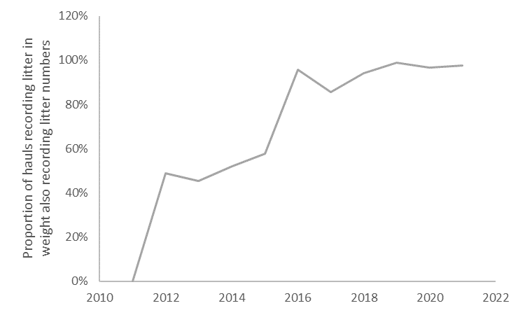
Figure 7. Development in the proportion of hauls recording litter in weight where number of litter items is also recorded.
Data are classified using one of the two formats C-TS (Original CEFAS trawl litter categories) and C-TS-REV (Revised CEFAS Trawl Litter Survey parameters). From 2019 onwards, only the latter of the two are used. The major categories are recorded in all years (plastic, metal, glass/ceramics, rubber, natural products and other) and are mutually exclusive (a litter item can only appear in one of these categories). Two further categories were also investigated (a litter item will appear in one of these categories only if it already appears in one of the above categories): Fisheries related plastic and Single Use Plastic (Table 8). The aim of this categorization is to reflect estimates of SUP and Fisheries related plastic as defined in EC (2019). As this represent a post hoc classification, the categories may contain litter that is not covered by the SUP Directive.
Table 8. Litter categorisation and assignment of categories to Single Use Plastic (SUP) and Fisheries related plastic. ‘Yes’ means the litter type is included in SUP or Fisheries related plastic. Litter categorised as SUP does not include Fisheries related plastic.
| C-TS | C-TS-REV | Type | SUP | Fisheries related plastic | |
| Plastic | A | A | Plastic | ||
| Plastic bottle | A1 | A1 | Plastic | Yes | |
| Plastic sheet | A2 | A2 | Plastic | Yes | |
| Plastic bag | A3 | A3 | Plastic | Yes | |
| Plastic caps | A4 | A4 | Plastic | Yes | |
| Plastic fishing line (monofilament) | A5 | A5 | Plastic | Yes | |
| Plastic fishing line (entangled) | A6 | A6 | Plastic | Yes | |
| Synthetic rope | A7 | A7 | Plastic | Yes | |
| Fishing net | A8 | A8 | Plastic | Yes | |
| Plastic cable ties | A9 | A9 | Plastic | ||
| Plastic strapping band | A10 | A10 | Plastic | ||
| Plastic crates and containers | A11 | A11 | Plastic | Yes | |
| Plastic diapers | B1 | A12 | Plastic | Yes | |
| Sanitary towel/tampon | B6 | A13 | Plastic | Yes | |
| Other plastic | A12 | A14 | Plastic | ||
| Sanitary waste (unspecified) | B | Plastic | Yes | ||
| Cotton buds | B2 | Plastic | Yes | ||
| Cigarette butts | B3 | Plastic | Yes | ||
| Condoms | B4 | Plastic | Yes | ||
| Syringes | B5 | Plastic | Yes | ||
| Other sanitary waste | B7 | Plastic | Yes | ||
| Metals | C | B | Metal | ||
| Cans (food) | C1 | B1 | Metal | ||
| Cans (beverage) | C2 | B2 | Metal | ||
| Fishing related metal | C3 | B3 | Metal | ||
| Metal drums | C4 | B4 | Metal | ||
| Metal appliances | C5 | B5 | Metal | ||
| Metal car parts | C6 | B6 | Metal | ||
| Metal cables | C7 | B7 | Metal | ||
| Other metal | C8 | B8 | Metal | ||
| Rubber | D | C | Rubber | ||
| Boots | D1 | C1 | Rubber | ||
| Balloons | D2 | C2 | Rubber | Yes | |
| Rubber bobbins (fishing) | D3 | C3 | Rubber | Yes | |
| Tyre | D4 | C4 | Rubber | ||
| Glove | D5 | C5 | Rubber | ||
| Other rubber | D6 | C6 | Rubber | ||
| Glass/Ceramics | E | D | Glass | ||
| Jar | E1 | D1 | Glass | ||
| Glass bottle | E2 | D2 | Glass | ||
| Glass/ceramic piece | E3 | D3 | Glass | ||
| Other glass or ceramic | E4 | D4 | Glass | ||
| Natural products | F | E | Natural | ||
| Wood (processed) | F1 | E1 | Natural | ||
| Rope | F2 | E2 | Natural | ||
| Paper/cardboard | F3 | E3 | Natural | ||
| Pallets | F4 | E4 | Natural | ||
| Other natural products | F5 | F5 | Natural | ||
| Miscellaneous | G | F | Other | ||
| Clothing/rags | G1 | F1 | Other | ||
| Shoes | G2 | F2 | Other | ||
| Other | G3 | F3 | Other |
9.2.2 Swept area corrections
The area swept was defined as the distance trawled multiplied by the width of the trawl between the wings. Data on wingspan, doorspread and distance travelled were not consistently available. Given the low proportion of hauls containing the necessary information to estimate the swept area for each haul, it was decided to instead assume that all hauls of a specific gear type covered the median of the swept areas estimated for all hauls with TVL and TVS, respectively (87163 m2 and 68184 m2, respectively).
9.2.3 Estimation of the indicator
Three metrics were investigated, the proportion of trawl hauls containing litter, the average catch of litter in number and the average catch of litter in weight, both per km2.
The statistical properties of the data (large overdispersion and occasional very large catches) necessitated analysing the data in a statistical model (Stefánsson 1996, Berg et al., 2014). Survey indices were therefore calculated using the methodology described by Berg et al. (2014). Three models were fitted for each type of litter to estimate the amount of litter caught. Model 1 assumes that the amount of litter develops smoothly from year to year as a result of litter deteriorating slowly in the wild. Hence, the model utilises the knowledge we have of the lifetime of litter on the seafloor and is considered the most appropriate model. Model 2 allows the amount of litter to change freely between years, equivalent to the assumption that litter is removed from the surveyed area every year and replaced by new litter. This model is equivalent to estimating the annual amount independently of the previous year and is commonly used. Model 3 estimates a linear trend over the period and can be used to evaluate if there has been a significant steady increase from year to year within the sampling period. An alternative method to investigate the development in litter over time could be to compare the level in the period from 2016 to 2021 with that in the period from 2010 to 2015. However, this test is less statistically strong than model 3 as it does not utilise the information present in the development within assessment periods and further is complicated by the sampling only beginning midway in the first assessment period for most countries.
The spatial distribution of litter was assumed constant over time due to the sparsity of data. The following equations describe the models:
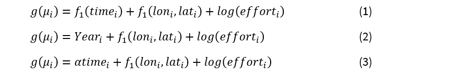
Effort is the swept area and amount caught is assumed to be directly proportional to this (i.e., if the area swept is doubled, the average amount caught is doubled). The swept area for a 30 min haul is assumed to be 68184 m2 for the TVS gear and 87163 m2 for the TVL (approx. 0.78 ratio, see above). All f-functions are Duchon splines with first derivative penalization. The models are fitted using both proportion of non-zero catches, numbers and mass as the response variable. For models using mass the Tweedie distribution (compound Poisson-Gamma) is used, because it is simple and easy to work with (see e.g., Thorson 2017). For models using numbers and to predict probability of catching litter the negative binomial distribution is used. Mass and number indices are standardized to a unit of kg / km2 or numbers / km2.
9.3 Monitoring and reporting requirements
There is a wide experience of collecting litter on the seafloor and fishing gear/lost fishing nets in the HELCOM area. Seafloor litter collection is integrated in bottom trawling for fish stocks assessment, so therefore the selection of the sampling stations as well as frequency is associated to the casuistic of the species of interest. Additional information can be found in the HELCOM Monitoring Programme on Litter on the Seafloor (HELCOM, 2020).
10 Data
The data and resulting data products (e.g., tables, figures and maps) available on the indicator web page can be used freely given that it is used appropriately, and the source is cited.
Data for use in the analysis were extracted from the ICES website (https://datras.ices.dk/Data_products/Download/Download_Data_public.aspx). The full code can be found here: https://github.com/DTUAqua/HELCOM-litter. The table below (Table 9) gives annual average values for each litter type and year.
Table 9. Annual model estimates of weight (mass) and number of litter items per km2 and probability of non-zero catch. Low and High denotes upper and lower 95% confidence intervals, respectively.
| Type | Year | Mass | MassLow | MassHigh | Numbers | NumbersLow | NumbersHigh | Prob | ProbLow | ProbHigh |
| Glass | 2012 | 0.44551 | 0.416846 | 0.605422 | 2.666697 | 2.049887 | 4.6012 | 0.118995 | 0.09691 | 0.159982 |
| Glass | 2013 | 0.445517 | 0.41552 | 0.599448 | 2.761062 | 2.193335 | 4.360735 | 0.121539 | 0.101878 | 0.152164 |
| Glass | 2014 | 0.445532 | 0.415663 | 0.603116 | 2.54682 | 2.11194 | 3.915167 | 0.115681 | 0.09878 | 0.144357 |
| Glass | 2015 | 0.445534 | 0.416347 | 0.601324 | 2.186015 | 1.773373 | 3.285524 | 0.105088 | 0.087959 | 0.131793 |
| Glass | 2016 | 0.445536 | 0.419242 | 0.58876 | 1.966743 | 1.637972 | 2.926399 | 0.098137 | 0.083707 | 0.122263 |
| Glass | 2017 | 0.445535 | 0.415385 | 0.610315 | 1.835458 | 1.576828 | 2.667841 | 0.093763 | 0.081616 | 0.11607 |
| Glass | 2018 | 0.44553 | 0.420258 | 0.595185 | 1.695945 | 1.487631 | 2.500857 | 0.088922 | 0.078073 | 0.109695 |
| Glass | 2019 | 0.445532 | 0.415355 | 0.590818 | 1.611645 | 1.422667 | 2.347476 | 0.085892 | 0.076074 | 0.105202 |
| Glass | 2020 | 0.445538 | 0.41616 | 0.600752 | 1.721922 | 1.504383 | 2.447111 | 0.089839 | 0.079622 | 0.10981 |
| Glass | 2021 | 0.445547 | 4.22E-01 | 0.602379 | 1.889319 | 1.645482 | 2.794938 | 0.095578 | 0.084314 | 0.117541 |
| Metal | 2012 | 0.278817 | 1.80E-01 | 0.619785 | 2.415496 | 1.713901 | 3.985435 | 0.129375 | 0.100189 | 0.172186 |
| Metal | 2013 | 0.385755 | 2.77E-01 | 0.748509 | 2.438146 | 1.893202 | 3.562842 | 0.130191 | 0.106718 | 0.161811 |
| Metal | 2014 | 0.480457 | 3.44E-01 | 0.944424 | 2.761709 | 2.133311 | 4.056337 | 0.141405 | 0.117079 | 0.173939 |
| Metal | 2015 | 0.509614 | 3.70E-01 | 0.99481 | 2.981882 | 2.376366 | 4.382549 | 0.148597 | 0.124847 | 0.181899 |
| Metal | 2016 | 0.595644 | 4.36E-01 | 1.119444 | 3.362414 | 2.761102 | 4.600896 | 0.16029 | 0.139066 | 0.188664 |
| Metal | 2017 | 0.974351 | 0.755916 | 1.832887 | 2.857335 | 2.435354 | 3.933275 | 0.14457 | 0.127348 | 0.171623 |
| Metal | 2018 | 0.847165 | 0.665291 | 1.509748 | 2.335822 | 1.98884 | 3.196872 | 0.126469 | 0.111147 | 0.152462 |
| Metal | 2019 | 0.82085 | 0.634643 | 1.569859 | 2.428742 | 2.073584 | 3.340907 | 0.129853 | 0.115408 | 0.154867 |
| Metal | 2020 | 1.149734 | 0.913114 | 2.191056 | 2.841842 | 2.437988 | 3.894713 | 0.144061 | 0.127789 | 0.170499 |
| Metal | 2021 | 1.267442 | 0.980223 | 2.323725 | 2.825967 | 2.436667 | 3.814477 | 0.143539 | 0.126694 | 0.169204 |
| Natural | 2012 | 3.620196 | 2.599513 | 6.138473 | 24.2258 | 14.8885 | 45.47056 | 0.286578 | 0.237343 | 0.344819 |
| Natural | 2013 | 6.270533 | 4.736894 | 10.2066 | 23.96556 | 17.84683 | 36.68562 | 0.285521 | 0.254387 | 0.319997 |
| Natural | 2014 | 8.589439 | 6.307281 | 13.89984 | 29.52924 | 21.91464 | 45.49308 | 0.30604 | 0.27112 | 0.343083 |
| Natural | 2015 | 6.089038 | 4.543524 | 10.13452 | 23.10761 | 16.67773 | 37.11972 | 0.281958 | 0.246298 | 0.3228 |
| Natural | 2016 | 1.945149 | 1.430028 | 3.262926 | 15.09974 | 11.76824 | 21.96961 | 0.241077 | 0.215729 | 0.270829 |
| Natural | 2017 | 1.498057 | 1.120274 | 2.472038 | 7.054283 | 5.498965 | 10.34529 | 0.173207 | 0.151964 | 0.200975 |
| Natural | 2018 | 2.554178 | 1.920114 | 4.064253 | 7.510614 | 5.737608 | 10.9563 | 0.178453 | 0.154115 | 0.204517 |
| Natural | 2019 | 4.383652 | 3.43986 | 6.727153 | 10.86231 | 8.541077 | 16.44772 | 0.210678 | 0.186863 | 0.239442 |
| Natural | 2020 | 4.559681 | 3.463246 | 6.994008 | 17.20075 | 13.74693 | 24.98245 | 0.253434 | 0.231349 | 0.281524 |
| Natural | 2021 | 3.029851 | 2.26182 | 5.000387 | 10.00476 | 7.804954 | 14.84023 | 0.203311 | 0.18126 | 0.230849 |
| Other | 2012 | 0.683721 | 0.514082 | 1.226198 | 2.058694 | 1.352842 | 3.764506 | 0.098831 | 0.07242 | 0.138985 |
| Other | 2013 | 0.73759 | 0.578255 | 1.239436 | 2.289719 | 1.695162 | 3.641892 | 0.105713 | 0.085119 | 0.135802 |
| Other | 2014 | 0.691079 | 0.549337 | 1.168765 | 2.746594 | 2.006484 | 4.240254 | 0.118162 | 0.096492 | 0.146931 |
| Other | 2015 | 0.711197 | 0.572256 | 1.177047 | 2.877021 | 2.147301 | 4.415927 | 0.121471 | 0.099127 | 0.151216 |
| Other | 2016 | 0.711995 | 0.569006 | 1.165453 | 2.872077 | 2.254205 | 4.201782 | 0.121347 | 0.102645 | 0.146192 |
| Other | 2017 | 0.72062 | 0.600031 | 1.149793 | 3.077284 | 2.490435 | 4.390988 | 0.126364 | 0.109725 | 0.149881 |
| Other | 2018 | 0.691668 | 0.556739 | 1.137364 | 2.698058 | 2.174886 | 3.826251 | 0.116905 | 0.101081 | 0.140103 |
| Other | 2019 | 0.809193 | 0.674828 | 1.287875 | 3.001113 | 2.486058 | 4.190662 | 0.124528 | 0.109374 | 0.146998 |
| Other | 2020 | 1.070679 | 0.887234 | 1.708392 | 4.342105 | 3.617725 | 6.02614 | 0.153068 | 0.134946 | 0.176797 |
| Other | 2021 | 1.19268 | 0.980058 | 1.885985 | 5.488249 | 4.559938 | 7.738453 | 0.172689 | 0.154007 | 0.19773 |
| Plastic | 2012 | 0.487681 | 0.373777 | 0.7207 | 24.87626 | 19.37626 | 33.8751 | 0.431346 | 0.39436 | 0.472188 |
| Plastic | 2013 | 0.943495 | 0.756934 | 1.368186 | 23.13959 | 19.14885 | 30.03497 | 0.42008 | 0.387667 | 0.452542 |
| Plastic | 2014 | 1.861788 | 1.484654 | 2.76175 | 24.9822 | 21.09779 | 32.1469 | 0.432008 | 0.403797 | 0.463863 |
| Plastic | 2015 | 2.247397 | 1.804174 | 3.089645 | 26.15674 | 22.08642 | 32.79934 | 0.439155 | 0.41077 | 0.468749 |
| Plastic | 2016 | 1.468015 | 1.208997 | 2.055911 | 26.17116 | 22.70678 | 32.16642 | 0.43924 | 0.415873 | 0.46509 |
| Plastic | 2017 | 1.432806 | 1.18836 | 1.998389 | 27.55173 | 24.08117 | 33.79315 | 0.447229 | 0.424877 | 0.472641 |
| Plastic | 2018 | 1.804394 | 1.53211 | 2.497888 | 26.60067 | 23.31656 | 32.00716 | 0.441771 | 0.41812 | 0.46523 |
| Plastic | 2019 | 2.300702 | 1.944203 | 3.106164 | 27.46569 | 24.31907 | 33.13106 | 0.446743 | 0.425114 | 0.471559 |
| Plastic | 2020 | 1.960626 | 1.642817 | 2.676456 | 31.11393 | 27.6549 | 37.41644 | 0.466062 | 0.443813 | 0.488021 |
| Plastic | 2021 | 1.405809 | 1.191638 | 1.938309 | 34.11683 | 29.81748 | 40.55215 | 0.480251 | 0.460134 | 0.501182 |
| Rubber | 2012 | 0.016701 | 0.006594 | 0.052692 | 1.320374 | 1.19597 | 1.783939 | 0.077265 | 0.070489 | 0.093145 |
| Rubber | 2013 | 0.040161 | 0.019895 | 0.110751 | 1.320382 | 1.172056 | 1.79269 | 0.077265 | 0.069534 | 0.092778 |
| Rubber | 2014 | 0.1163 | 0.057237 | 0.305315 | 1.320377 | 1.176659 | 1.788766 | 0.077265 | 0.0694 | 0.092985 |
| Rubber | 2015 | 0.252998 | 0.146836 | 0.582245 | 1.320359 | 1.18573 | 1.794996 | 0.077264 | 0.069904 | 0.092653 |
| Rubber | 2016 | 0.334959 | 0.206005 | 0.745389 | 1.32034 | 1.18767 | 1.785075 | 0.077263 | 0.069849 | 0.093129 |
| Rubber | 2017 | 0.231329 | 0.14576 | 0.524223 | 1.320283 | 1.177214 | 1.774076 | 0.077261 | 0.069883 | 0.092427 |
| Rubber | 2018 | 0.28724 | 0.181615 | 0.594962 | 1.320263 | 1.184293 | 1.803505 | 0.07726 | 0.070016 | 0.09243 |
| Rubber | 2019 | 0.784377 | 0.525989 | 1.614402 | 1.32028 | 1.184322 | 1.798943 | 0.077261 | 0.070471 | 0.093248 |
| Rubber | 2020 | 1.033477 | 0.682844 | 2.232517 | 1.320312 | 1.170545 | 1.772362 | 0.077262 | 0.069443 | 0.09207 |
| Rubber | 2021 | 0.543547 | 0.337187 | 1.14843 | 1.320321 | 1.169866 | 1.784994 | 0.077263 | 0.069823 | 0.092858 |
| SUP | 2012 | 0.000839 | 0.000348 | 0.002243 | 2.733454 | 1.724973 | 4.700086 | 0.160279 | 0.112993 | 0.226453 |
| SUP | 2013 | 0.252307 | 0.189019 | 0.407648 | 6.605985 | 5.217605 | 8.963356 | 0.279195 | 0.240493 | 0.325725 |
| SUP | 2014 | 0.410478 | 0.304204 | 0.660197 | 10.08766 | 7.659662 | 14.37608 | 0.346741 | 0.299268 | 0.398796 |
| SUP | 2015 | 0.260502 | 0.192654 | 0.404333 | 11.12199 | 8.652187 | 15.38066 | 0.362867 | 0.316569 | 0.412637 |
| SUP | 2016 | 0.474416 | 0.384744 | 0.707176 | 10.96174 | 9.382525 | 13.95706 | 0.36046 | 0.330191 | 0.396746 |
| SUP | 2017 | 0.546632 | 0.446862 | 0.808481 | 10.58062 | 9.143428 | 13.2179 | 0.354605 | 0.327293 | 0.38498 |
| SUP | 2018 | 0.693842 | 0.567204 | 1.003291 | 9.241721 | 7.762919 | 11.82625 | 0.33241 | 0.300577 | 0.366714 |
| SUP | 2019 | 0.847749 | 0.70014 | 1.197004 | 11.31024 | 9.873038 | 14.08182 | 0.365653 | 0.338682 | 0.397834 |
| SUP | 2020 | 0.86729 | 0.69867 | 1.235669 | 13.22162 | 11.44637 | 16.65218 | 0.391722 | 0.362727 | 0.425082 |
| SUP | 2021 | 0.814305 | 0.659653 | 1.153089 | 10.81527 | 9.439988 | 13.41733 | 0.358232 | 0.33107 | 0.392356 |
| Fishing.related | 2012 | 0.016902 | 0.008027 | 0.053815 | 1.822417 | 1.017337 | 3.420608 | 0.084898 | 0.056947 | 0.12152 |
| Fishing.related | 2013 | 0.058469 | 0.034531 | 0.147072 | 2.266205 | 1.553602 | 3.814894 | 0.097413 | 0.075346 | 0.12901 |
| Fishing.related | 2014 | 0.25091 | 0.142648 | 0.633787 | 3.330431 | 2.256848 | 5.423839 | 0.1222 | 0.096323 | 0.156589 |
| Fishing.related | 2015 | 0.346305 | 0.202241 | 0.85014 | 4.777329 | 3.300204 | 7.479029 | 0.148297 | 0.121855 | 0.180101 |
| Fishing.related | 2016 | 0.222457 | 0.15339 | 0.508151 | 4.819838 | 3.620443 | 6.991735 | 0.14897 | 0.12868 | 0.176014 |
| Fishing.related | 2017 | 0.167531 | 0.110093 | 0.369704 | 4.83173 | 3.741497 | 6.968711 | 0.149157 | 0.13003 | 0.174202 |
| Fishing.related | 2018 | 0.417742 | 0.292502 | 0.936551 | 4.733385 | 3.749024 | 6.69322 | 0.147597 | 0.128089 | 0.171707 |
| Fishing.related | 2019 | 0.879136 | 0.626643 | 1.812058 | 3.659236 | 2.853184 | 5.14664 | 0.128757 | 0.110982 | 0.15063 |
| Fishing.related | 2020 | 0.74537 | 0.527651 | 1.584376 | 5.286768 | 4.219909 | 7.496612 | 0.156074 | 0.137205 | 0.180269 |
| Fishing.related | 2021 | 0.529883 | 0.365336 | 1.112158 | 6.305216 | 5.029919 | 8.796378 | 0.170013 | 0.150109 | 0.192499 |
11 Contributors
Anna Rindorf, Marie Storr-Paulsen
HELCOM Expert Group on Marine Litter (HELCOM EG Marine Litter).
HELCOM Secretariat: Jannica Haldin, Owen Rowe, Marta Ruiz
12 Archive
This version of the HELCOM core indicator report was published in April 2023:
The current version of this indicator (including as a PDF) can be found on the HELCOM indicator web page.
No earlier versions currently exist.
13 References
Barnes D.K.A, Galgani F., Thompson R.C, Barlaz M. 2009. Accumulation and fragmentation of plastic debris in global environments. Philos. Trans. R. Soc. Lond. B Biol. Sci 364: 1985–1998. doi: 10.1098/rstb.2008.0205.
Berg, C. W., Nielsen, A., Kristensen, K. 2014. Evaluation of alternative age-based methods for estimating relative abundance from survey data in relation to assessment models. Fisheries research, 151, 91-99.
Bergmann M., Klages M. 2012. Increase of litter at the Artic deep-sea observatory HAUSGARTEN. Marine Pollution Bulletin, 64, 2734-2741.
Brown, J, G. Macfadyen, T. Huntington, J. Magnus and J. Tumilty (2005). Ghost Fishing by Lost Fishing Gear. Final Report to DG Fisheries and Maritime Affairs of the European Commission. Fish/2004/20. Institute for European Environmental Policy / Poseidon Aquatic Resource Management Ltd joint report.
Derraik J.G.B. 2002. The pollution of the marine environment by plastic debris: a review. Marine Pollution Bulletin 44, 842–852.
Galgani F., Leaute J.P., Moguedet P., Souplet A., Verin Y., Carpentier A., Goraguer H., Latrouite D., Andral F., Cadiou Y., Mahe J.C., Poulard J.C., Nerisson P. 2010. Litter on the Sea Floor Along European Coasts. Marine Pollution Bulletin, 40 (6) 516-527.
Galgani F., Hanke G., Maes T.. 2015. Global Distribution, Composition and Abundance of Marine Litter. In: Bergmann M. et al (eds): Marine anthropogenic litter. Springer Open. pp 29-56.
Goldberg E.D. 1994. Diamonds and plastics are forever? Marine Pollution Bulletin 28, 466.
HELCOM, 2013. HELCOM Copenhagen Declaration “Taking Further Action to Implement the Baltic Sea Action Plan – Reaching Good Environmental Status for a healthy Baltic Sea”. Online August 2014 http://www.helcom.fi/Documents/Ministerial2013/Ministerial%20declaration/2013%20Copenhagen%20Ministerial%20Declaration%20w%20cover.pdf
HELCOM 2020. HELCOM Monitoring Programme on Litter on the Seafloor. https://helcom.fi/wp-content/uploads/2020/10/MM_Litter-on-the-seafloor.pdf
HELCOM Recommendation 42-43/3, 2021. Regional Action Plan on Marine Litter. https://helcom.fi/wp-content/uploads/2021/10/Rec-42-43-3.pdf
ICES. 2014. Manual for the Baltic International Trawl Surveys (BITS). Series of ICES Survey Protocols SISP 7 – BITS. 71 pp.
ICES. 2015. Manual for the International Bottom Trawl Surveys. Series of ICES Survey Protocols SISP 10 ‐ IBTS IX. 86 pp.
ICES. 2022. ICES Manual for Seafloor Litter Data Collection and Reporting from Demersal Trawl Samples. ICES Techniques in Marine Environmental Science (TIMES). Report. https://doi.org/10.17895/ices.pub.21435771.v1.
JRC, 2013. Guidance on Monitoring of Marine Litter in European Seas. Online August 2014 http://publications.jrc.ec.europa.eu/repository/bitstream/111111111/30681/1/lb-na-26113-en-n.pdf.
Katsanevakis, S. 2008. Marine debris, a growing problem: Sources, distribution, composition, and impacts. In: Hofer TN (ed) Marine Pollution: New Research. Nova Science Publishers, New York. pp. 53–100.
Lundqvist, J. 2013 . Quantification of debris on the seafloor in shallow (<20 m) areas using a towed video camera system, Report of university of Gothenburg, Faculty of sciences, pp. 22.
Majaneva & Suonpää, 2015. Vedenalaisen roskan kartoitus Helsingin edustan merialueella – pilottiprojekti. http://www.hel.fi/static/ymk/julkaisut/julkaisu-02-15.pdfa
MARELITT, 2019. https://www.marelittbaltic.eu/
Mordecai, G., Tyler, P.A., Masson, D.G., Huvenne, V.A.I., 2011. Litter in submarine canyons off the west coast of Portugal. Deep Sea Res. Part II 58, 2489.
Moret-Ferguson, S., Law, K.L., Proskurowski, G., Murphy, E.K., Peacock, E.E., Reddy, C.M., 2010. The size, mass, and composition of plastic debris in the western North Atlantic Ocean. Marine Pollution Bulletin 60, 1873–1878.
Miyake H., Shibata H., Furushima Y. 2011. Deep-sea litter study using deep-sea observation tools. In: Omori K., Guo X., Yoshie N., Fujii N., Handoh I.C. et al., editors. Interdisciplinary Studies on Environmental Chemistry-Marine Environmental Modeling and Analysis: Terrapub. pp. 261–269.
Newman S., Watkins E., Farmer A., ten Brink P., Schweitzer J.P. 2015. The Economics of Marine Litter. Chapter 14 in: Marine Anthropogenic Litter, Eds. Bergmann M., Gutow L., Klages M., Eprint ID 37207 of the Alfred-Wegener-Institut Helmholtz-Zentrum für Polar- und Meeresforschung, Springer Open Publication, 447pp.
OSPAR, 2022. OSPAR’s Second Regional Action Plan for the Prevention and Management of Marine Litter in the North-East Atlantic (2022-2030) http://www.ospar.org/documents?v=48461
Pace, R., Dimech, M., Camilleri, M., Schembri, P.J., Briand, F., 2007. Litter as a Source of Habitat Islands on Deepwater Muddy Bottoms. CIESM, Monaco.
Pham C.K., Ramirez-Llodra E., Alt C.H.S., Amaro T., Bergmann M., Canals M., Company J.B., Davies J., Duineveld G., Galgani F., Howell K.L., Huvenne V.A.I., Isidro E., Jones D.O.B., Lastras G., Morato T., Gomes-Pereira J.N., Purser A., Stewart H., Tojeira I., Tubau X., Van Rooij D., Tyler P.A. 2014. PLoS ONE 9(4): e95839. doi:10.1371/journal.pone.0095839.
Stefánsson, G. 1996. Analysis of groundfish survey abundance data: combining the GLM and delta approaches. ICES journal of Marine Science, 53(3), 577-588.
Thompson R.C. 2006. Plastic debris in the marine environment: consequences and solutions. In: Krause, J.C., Nordheim, H., Bräger, S. (Eds.), Marine Nature Conservation in Europe. Bundesamt für Naturschutz, Stralsund, Germany, 107–115.
Ye S. & Andrady A.L. 1991. Fouling of floating plastic debris under Biscayne Bay exposure conditions. Marine Pollution Bulletin 22, 608–613.
14 Other relevant resources
No additional information is currently required.